 continued...
This page covers analytical work related to data in the POCAL coverage of DNRGIS data for the Washougal River watershed.
The POCAL file contains information relating to land use, land cover, timber cruise data (dbh, species, stand orgination date), public land survey markers, and ownerships.
This page presents information on Tree Height Calculation using the POCAL and SOILS layers, as well as a variety of maps based on land use, land cover, and stand origin data extracted from POCAL and various associated coverages.
Two data dictionaries exist for the POCAL coverage. Download them here:
pocal.doc DNR POCAL data dictionary
lulc.doc DNR LULC data dictionary
The following, from a memo provided by Weikko Jaross,
describes the process of estimating tree height based upon available species,
age and site index data.
Getting tree height for estimating stream shade is a complex
process. DNRGIS does not provide an estimate of tree height. Therefore
one must estimate it. The best way to do this is to use regression equations
based on species, age, and site index. Remember that site index is an estimate
of the tree height in feet at age 50 or 100 years. These equations require
the variables, age, and site index for a given species. The following are
examples of equations:
Equations for Estimating Tree Height of Merchantable
West-Side Timber:
Western Hemlock (Wily)
A = age @ Breast Height
Z = 2500 / (50-yr site index 4.5)
Height = A * A / (-1.7307 + .1394 * Z + (-.0616 + .0317
* Z) * A + (.00192 + .00007 * Z) * A *A) + 4.5
Western Hemlock (Ministry of Forestry, Victoria, B.C.)
(more accurate)
A = age @ Breast Height
Height = 2.2226 * (1 - e^(-0.0174 * A))^1.4711
Douglas fir (King)
A = age @ Breast Height
Z = 2500 / (50-yr site index 4.5)
Height = A * A / (-.9540 + .1098 * Z + (-.0616 + .0317
* Z) * A + (-.0007 + .0002 * Z) * A *A) + 4.5
Silver fir (Hoyer & Herman)
A = age @ Breast Height
SI = 50-yr site index
Height = 4.5 + (SI 4.5) * (1-1 / 2.7183 ^ (.0051 + .000091313
* (SI 4.5) * A)) * (1.1053 / 1 1 / (.0051 + .000091313 *
(SI 4.5) * 50)) * 1.1053
Silver Fir (Hoyer) (more
accurate)
c = .0071839
d = .0000571
f = 1.39005
A = age @ Breast Height
SI = 50-yr site index
Height = (4.5+(SI-4.5) * ((1-exp(-(c+d*(SI-4.5))*A))^f)) / ((1-exp(-(c+d*(SI-4.5))*50))^f)
Red alder (Worthington)
A = age @ Breast Height
SI = 50-yr site index
Height = SI / (.6092 + 19.538 / A)
Below is the method used to join site index, stand origin and species data from the various coverages provided in DNRGIS:
The variables age, site index and species are kept in several different sources in DNRGIS. The procedure to collect this information for a given stand of timber requires several steps. First collect your information. FTP and import into your workspace the DNRGIS covers POCAL.PAT (40), POCAL.45, and POCAL.46 and SOILS.PAT (30) and SOILS.MAIN (35). The general procedure is to relate the PAT files with the age, species, and site index from the info files with specific items. Complete the following process for the POCAL cover using ARC and ARCEDIT commands.
Relate or join POCAL.PAT (40), POCAL.45, and POCAL.46 using the item STAND.NO. For example You will need the items PRI.SPEC (species) from LULC.COM (POCAL.45) and PRI.ORIG (year of origin) from LULC.EVEN (POCAL.46). Refer to the DATA DICTIONARY for information regarding the LULC cover and tables. You now have a POCAL polygon coverage with the age and species items.
The next step is to relate or join the site index information to the spatial information in the SOIL cover. To accomplish this relate the SOILS.PAT (30) and SOILS.MAIN (35) using the item ST.SOIL.SYM. You now have spatial information regarding the item SITE.INDEX.SIDE. Note that some indexes for "eastside" soils are base on the 50 year index table. Check the Data Dictionary regarding the SOILS cover for more information.
Now that we have two covers with the variables to calculate tree height, you need to assign them to the unique timber stand polygons. To accomplish this overlay the related SOILS.PAT cover with the item SITE.INDEX.SIDE onto the POCAL.PAT with the items PRI.ORIG and PRI.SPEC. This step will assign the site index to the POCAL polygons. Simplify your new PAT file by having the only the species, age, and site index items.
The last step is to calculate tree height. Add a new item
called TREE.HT to the new PAT file. Use the above mentioned equations for
the particular species in each record. Now you have a polygon coverage
with species, age, site index, and estimated height.
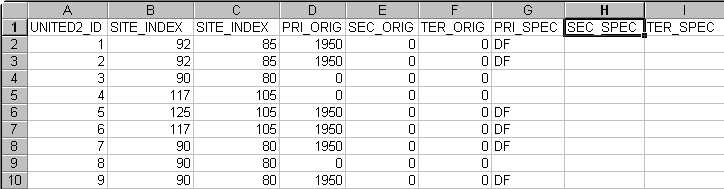
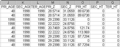
Spreadsheet analysis was then used to calculate tree height
data from the joined tables.
A Microsoft Excel spreadsheet was used to solve the tree
height equations listed above. Tables were imported from ARC into
Excel using the highly compatible *.dbf dBASE format. Approximately
1000 polygon data records were processed within the Washougal watershed
spreadsheet. This analysis provided quick and generally accurate
results. Site index, stand origin, species data, and Z value equations
(given above) were combined in a deeply nested conditional statement, here
presented verbatim:
=IF(B2<1,0,IF(D2<1,0,IF(G2="DF",((J2^2/((-0.954038+0.109757*M2)+(0.0558178+0.00792336*M2)*
J2+(-0.000733819+0.000197693*M2)*J2^2))+4.5),IF(G2="RA",(B2/(0.6092+19.538/J2)),
IF(G2="WH",(2.2226*B2*(1-EXP(-0.0174*J2))^1.4711),IF(G2="SF",(4.5+(B2-4.5)+
((1-EXP(-(0.0071839+0.0000571*(B2-4.5))*J2))^1.39005)/((1-EXP(-(0.0071839+0.0000571*(B2-4.5))*50))^1.39005)),0))))))
The tables from our analysis, in spreadsheet form, looked
like this:
continued...
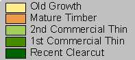
MAP OF STAND ORIGIN DATA:
Here is a map based on the pri.orig data provided
in pocal. Pri.orig is the date of origination
of the stand. From this data, Candace and I were able to determine
the age class of the given stands.
Old Growth:
ORIGINATION: 1900 and earlier
-much of this may be harvestable if not
locked-up
Mature Timber:
ORIGINATION: between 1901 - 1938
-mature stands ready for harvest
2nd Commercial Thin:
ORIGINATION: between 1939
- 1958
-these stands are due for a second commercial
thin
1st Commercial Thin:
ORIGINATION: between 1959 - 1978
-these stands are due for a first commercial
thin
Recent Clearcut:
ORIGINATION: 1979 - Present
-may include regeneration / reprod
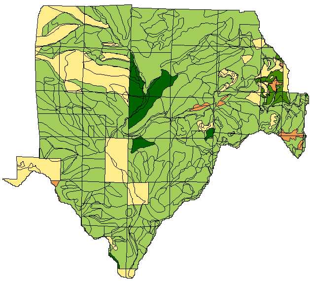
MAP OF LAND USE:
Below is a map of land uses in the Washougal area. Note the
large proportion of 'natural even age stand management' within the area.
This is a result of the Yacolt Burn. In the northwestern and central portions
of this map, there are inoperable areas, and areas with low-site forestland.
MAP OF LAND COVER:
This map shows the 8 primary types of land cover which occur
in the Washougal drainage. Primarily, the land is in a forested state,
though areas of exposed rock and soil are common. Yes, there is a
small exposed surface mine, though it is not visible here on this page.
The data derived from this analysis could potentially be used to create stand visualizations and projections using a forest vegetation simulator. Perhaps the most comprehensive tool available for analyzing and visualizing the stand data is the Landscape Management System (LMS), produced under the direction of Chadwick D. Oliver at the Silivicuture Laboratory of the University of Washington College of Forest Resources.
According to the LMS web site:
The Landscape Management System (LMS) is an evolving set of software tools being designed to aid in landscape level management. LMS is being developed as part of the Landscape Management Project at the Silviculture Laboratory, College of Forest Resources, University of Washington.
Landscape Management System (LMS) is a computerized system that integrates landscape-level spatial information, stand-level inventory data, and distance-independent individual tree growth models to project changes through time across forested landscapes. LMS facilitates forest management, planning, policy-making, as well as education.
LMS coordinates the execution and information flow between 20-plus programs. These programs: format, classify, summarize, and export information; project tree growth and snag decay; manipulate stand inventories; and present stand- and landscape-level visualization and graphics.
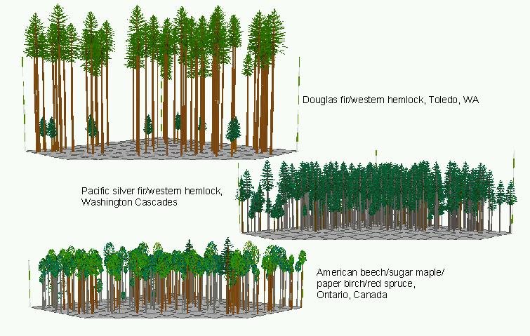
Due to time constraints, vegetation simulation was
not conducted during this analysis of the Washougal LULC data.
Provided below are examples of visualizations created by LMS and its associated
software.
An LMS / SVS stand visualization with terrain modeling:
An example of ground-level visualization of stand data from LMS: