Appendix A

In the course of doing harvest and road design, it becomes necessary to develop profiles for skyline analysis and road design, especially in the early planning phases. A common starting point for both these activities is a contour map. For some agencies, the best contours are derived from 10m USGS digital elevation models, whereas at least for the Department of Natural Resources the best contours are produced from photogrammetry and published on 1": 400' maps. However, even with these contours a significant amount of time is spent in the field taking measurement for skyline and road profiles. Lidar-based digital elevation models, though, are setting a new standard for accurate elevation data (and hence accurate contours). If we want to see what we gain by using lidar elevation data, we need to know what problem we are trying to solve by collecting field data in the first place. The question then is basically "what do we get out of field work that we cannot get out of current contour maps?"

With field work, then, we are essentially seeking a measure of confidence in our data by doing a survey or traverse where error may be computed and known. A given activity may require a certain degree of precision, and thus defines a certain set of equipment and amount of time to be used to conduct that activity. In the case of running a skyline profile, a string box and clinometer may be sufficient.

Why would we need to seek confidence? In the case where we need accurate vertical data, such as the case of a road centerline traverse, it would seem that the 10m DEM only gives us enough detail to get a general sense of landforms, but not enough to do design work. The 1": 400' contours are better, but they are only contours on paper maps. To be of real use in planning, they would be derived from another DEM. However, that is not the case, although one could digitize the contours and create a TIN from that. That would be exceptionally time consuming, mostly for adding the elevation attributes and edgematching the different sheets together. Further, the 1":400' contours still miss features such as small benches that need to be captured if one is to reduce the amount of time spent in the field.

As an example of these issues, we have a profile for a field-run cable road from the Schwing sale. It was run with a clinometer and string box to get the slope breaks from the landing to the road below. Looking at the 1": 400' contours to the right in Figure x, one can see something of a bench about halfway down the profile. Yet it doesn't seem like a large enough bench to really make much of a difference to skyline deflection. Obviously, then, there was something else there to necessitate running a field profile, something the standard contours missed. Looking at the lidar-based 20' contours to the left in Figure 1 shows quite clearly why the profile was run in the field. Follow the arrow and notice the more pronounced bench.

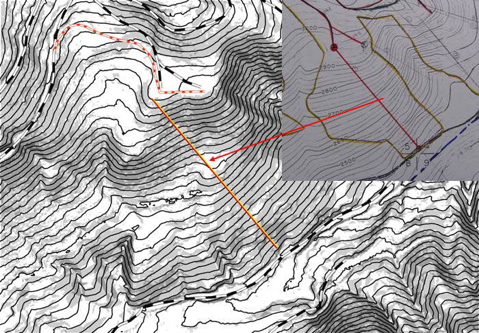
Figure 1: The arrow points from a small bench on the contours to the right to a more pronounced bench on the contours and slope classes to the left. The figure shows the location of a field profile run for the Schwing Timber Sale, and then draped over two different DEM's to compare with the field profile.

Now, running profiles in the field is a time consuming process. If a way can be found to eliminate the need to run them using GIS technology and lidar-based elevation data, then that would save rather a lot of time for field staff.

One process to do this was fairly straightforward. We started with a digital elevation model (DEM) and draped a shapefile line over that in order to assign a Z-value, using ArcMap's 3D Analyst extension. The new shapefile created by this process could then be converted into a 3D DXF polyline and imported into RoadEng. From there, we built an ASCII file of survey stations and elevations. This was imported into TDS ForeSight to create another DXF file that could be used in AutoCAD. The last two steps were done to compare the field, 10m, and lidar profiles easily. One could potentially stop at RoadEng and use its cable-analysis package, as well as do any necessary preliminary road design.

The results of the operation can be seen in Figure 2. One can immediately see that there is a large difference between the lidar and 10m DEM's. As well, looking at the field profile suggests that the lidar does indeed catch the bench in question more accurately than does the 10m DEM. However, there is still a matter of some discrepancies between the beginning and ending points between the lidar and field profiles. These might be explained by a difference in starting points, resulting in a shift from where the field profile was actually run. A way to remedy this would be to simply take a GPS point whenever starting a field profile, so that there would be no question as to where the profile actually starts.

Figure 2: The blue line is a field-run profile from the Schwing Sale, run with a string box and clinometer. The other two lines are profiles created by draping a straight line over a 10m DEM and lidar-based DEM. Although there are some discrepancies between the field profile and the lidar profile at the beginning and end, the lidar catches a bench nicely. The differences may be explained by an inconsistent starting point between the GIS line and the field profile.

We also looked at the Closer Road profile, which has a known starting point. This road was traversed with a Criterion and staff compass, and closed at 1:700. Figure 3 shows the area of interest, with the red and white dashed line being the road alignment. The contours (at a 20' interval) were generated from a standard 10m DEM. Underneath are a hillshade and slopeclasses from the lidar-derived DEM. The yellow circles highlight those areas where the 10m DEM misses features caught by the lidar. One of these features, a bench by the main draw, has an important effect on result of draping the alignment over the 10m DEM.

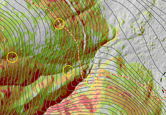
Figure 3: This figure shows the general vicinity of the Closer Road, which was traversed with a Criterion and staff compass. The contours were generated from a 10m DEM, whereas the slope classes (colors) were generated from a lidar-based DEM. Just by looking at the contours, one may see where the 10m DEM misses details picked up by the lidar coverage. The circles represent places where the 10m DEM misses features picked up by the lidar coverage.

The profiles seen in Figure 4 are part of the same stretch of road seen in Figure x above. Note the pronounced hump on the 10m DEM profile (top line), which was caused when the DEM missed a bench that is actually there. On the other hand, the lidar (middle line) caught the bench and tracks nicely with the field profile. Given this level of accuracy, one could very well do a preliminary road design before going out into the field.

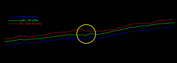
Figure 4: This figure compares three profiles over the same stretch of road alignment from the Closer design. The top profile represents the horizontal alignment draped over the standard 10m DEM. The middle profile represents the road alignment draped over the new lidar-based DEM. The bottom profile is the actual field survey conducted with a Criterion laser EDM and staff compass. Overall, the lidar and field profiles agree rather well. The 10m DEM profile misses a bench by the stream crossing (towards the middle of the profile), resulting in the pronounced hump not seen on the other two profiles.

These issues highlight what one can gain by using lidar data. With lidar-based digital terrain models, we essentially gain confidence in elevation data, to the degree that preliminary road design work could be done before going out to the field, as well as potentially eliminate the need to run field skyline profiles. All this points to savings in the amount of time spent in the field.

As well, with this improved data PLANS (Preliminary Logging ANalysis System) becomes the skyline analysis program of choice, rather than LoggerPC. The advantage PLANS has over LoggerPC is that where LoggerPC is a one-at-a-time cable analysis program, PLANS can analyze entire settings with as many corridors as the user wants very quickly and easily. As well, PLANS data can be exported fairly easily to Arc/Info for use in displaying on maps, which works better for doing harvest planning. PLANS also makes use of a digital terrain model, whereas LoggerPC depends on some manner of direct input, be it by keyboard, ASCII file, or manual digitizing.

Lidar also helps to speed up road planning, especially with the use of the ArcView extension "Pegger," which saves time over traditional paper-based road pegging.

There are some limitations as what one can do with lidar data, though. Most critical areas that one seeks to avoid in road location activities have some sort of surface expression, such as draw, slumps, wet areas, or rock outcrops. Draws and slumps can be picked up by lidar since they have a surface expression defined by their shape on the ground. However, a wet area or a rock outcrop aren't typically defined by their shapes alone, and so won't necessarily be picked up by lidar. This is important, since going through wet areas often demands greater construction costs and high maintenance costs, both something that should be minimized as much as possible. So, even if one can do a good preliminary design based on lidar data, there is still a strong potential of finding a "surprise" in the field that can change a small portion of the design or the whole thing altogether in order to mitigate or avoid a "surprise."

This leads to the aspect of "false positives." Now, lidar is generally better than 10m DEMS or 1": 400' contours. But the fact that it doesn't show everything that can surprise one in the field can lead to the false positive notion that the feature to be avoided is not actually there. So, field work and aerial photo interpretation are still necessary to catch things like wet spots and rock outcrops. In the case of the Closer Road, we had to shift the alignment uphill a ways in order to avoid putting the road on and below an old railroad grade, since intercepts a lot of water and the terrain below is wet and steep. With the lidar data, we could tell that the terrain below the grade was steep, but didn't find out it was wet until we actually started setting the gradeline.

Finally, getting a laser beam through dense vegetation, especially stands in stem exclusion, can be problematic. In these sort of areas, this typically leads to good ground return points spaces farther apart, which leads to a surface that has a more triangular look to it. This in turn can lead to lower confidence in elevation data for those areas.

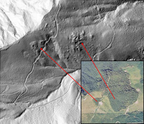
Figure 5: The red arrows point from stands in the aerial photo to their corresponding locations on the lidar-derived hillshade. Note that these stands, as shown in the photo, are denser than those around them. The hillshade shows by way of a rougher, triangular surface that there were fewer laser returns off the ground in those stands. Also note the representation of the ground in the adjacent stands and clearcuts.