Contents

Example applications of the bootstrap method

Applying the basic bootstrap method is really straightforward. The only messy part is doing the 'bias-corrected and accellerated' correction (BCa)on the confidence interval. I've provided a function called 'bootstrap' that runs the bootstrap algorithm and then (by default) does the BCa correction. In many cases, this correction doesn't make much difference and in some of the examples below I don't even know how to apply it, so I've left it out.

The examples below run through a series of fairly simple applications of the bootstrap method on statistics that we may or may not have a table for.

clear all

Example 1: Bootstrapping instead of a t-test (with unequal sample sizes)

A t-test tests the hypothesis that two samples come from the same distribution based on the differences between the means of the samples. T-tests assume the usual stuff about normal distributions and are most commonly used when comparing equal sized samples. When comparing samples of different sizes, an estimate of pooled variance is used, and the degrees of freedom are the average of the two df's from each sample. This seems like a bit of a hack to me.

To bootstrap on samples, we'll sample with replacement from both samples. Just as with the ratio of variances example below, allowing for different sample sizes means that we can't use the BCa method. We'll do the bootstrapping by hand again without the 'bootstrap' function.

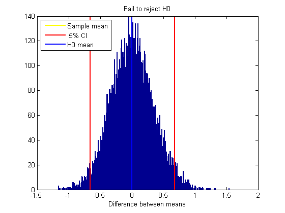
In this specific example we'll test the hypothesis that the means are different (a two-tailed test).

nReps = 10000;
n1 = 30;            %sample size 1
n2 = 15;            %sample size 2
alpha = .05;        %alpha value

generate fake data by drawing from normal distributions

x1 = randn(n1,1);
x2 = randn(n2,1);

define the statistic as the difference between means

myStatistic = @(x1,x2) mean(x1)-mean(x2);

sampStat = myStatistic(x1,x2);
bootstrapStat = zeros(nReps,1);
for i=1:nReps
    sampX1 = x1(ceil(rand(n1,1)*n1));
    sampX2 = x2(ceil(rand(n2,1)*n2));
    bootstrapStat(i) = myStatistic(sampX1,sampX2);
end

Calculate the confidence interval (I could make a function out of this...)

CI = prctile(bootstrapStat,[100*alpha/2,100*(1-alpha/2)]);

%Hypothesis test: Does the confidence interval cover zero?
H = CI(1)>0 | CI(2)<0;

Draw a histogram of the sampled statistic

clf
xx = min(bootstrapStat):.01:max(bootstrapStat);
hist(bootstrapStat,xx);
hold on
ylim = get(gca,'YLim');
h1=plot(sampStat*[1,1],ylim,'y-','LineWidth',2);
h2=plot(CI(1)*[1,1],ylim,'r-','LineWidth',2);
plot(CI(2)*[1,1],ylim,'r-','LineWidth',2);
h3=plot([0,0],ylim,'b-','LineWidth',2);
xlabel('Difference between means');

decision = {'Fail to reject H0','Reject H0'};
title(decision(H+1));
legend([h1,h2,h3],{'Sample mean',sprintf('%2.0f%% CI',100*alpha),'H0 mean'},'Location','NorthWest');

Example 2: Bootstrapping on an 'index'

Often (especially in neuroscience) we make up our own 'index' that is a measure of the effect of a condition on our measure. For example, when measuring neuronal firing rates, comparing the difference in firing rates between two conditions is often expressed as an index that is the ratio of the difference over the sum of the two firing rates. This normalizes by the overall firing rate of the neuron and provides a number that is always between -1 and 1.

In this example, we'll make up two samples of 25 firing rates corresponding to 25 neurons measured in two conditions. We'll then calculate the index for each neuron and bootstrap on mean of the indices to see if it is different from zero.

n=25;                   %number of neurons
nReps = 10000;          %number of iterations for the bootstrap
CIrange = 95;           %confidence interval range

x = ceil(15*randn(n,2).^2);      %nx2 matrix of firing rates (Chi-squared distribution)

define our 'index' here (difference over sum)

myStatistic = @(x) mean((x(:,1)-x(:,2))./(x(:,1)+x(:,2)));

run the 'boostrap' program to generate the confidence interval

[CI,sampStat,bootstrapStat] = bootstrap(myStatistic,x,nReps,CIrange);

Show the histogram of the boostrapped indices

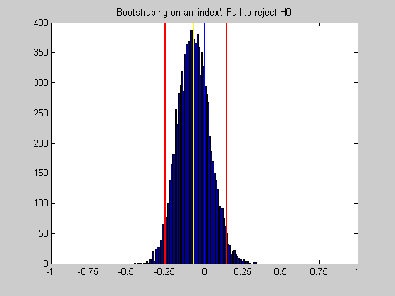
figure(1)
clf

xx = min(bootstrapStat):.01:max(bootstrapStat);
hist(bootstrapStat,xx);
hold on
ylim = get(gca,'YLim');
plot(sampStat*[1,1],ylim,'y-','LineWidth',2);
plot(CI(1)*[1,1],ylim,'r-','LineWidth',2);
plot(CI(2)*[1,1],ylim,'r-','LineWidth',2);
plot([0,0],ylim,'b-','LineWidth',2);
set(gca,'XTick',[-1:.25:1]);
set(gca,'XLim',[-1,1]);

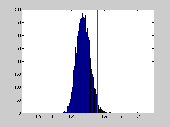
If our confidence interval does not include zero, then we'd conclude that the mean of our indices across the neurons is significantly different from zero.

H = CI(1)>0 | CI(2)<0;
title(sprintf('Bootstraping on an ''index'': %s',decision{H+1}));

Exercise: Add a value to the first column to see if you can reject the null hypothesis.

Example 3: Bootstrapping on a ratio of variances

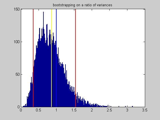
A ratio of variances of two samples an F-distribution. An F-test tests the null hypothesis that the two variances are the same (ratio = 1). We can perform a nonparametric version of the f-test using the bootstrap method.

CIrange = 90;
nReps = 10000;
n1 = 20;
n2 = 100;

two draws from a unit normal distribution

x1 = randn(n1,1);
x2 = randn(n2,1);

Our statistic is the ratio of the variances

myStatistic = @(x1,x2) var(x1)/var(x2);

This is our observed value (should be near 1)

sampStat = myStatistic(x1,x2);

We'll do this manually, rather than call the boostrap program because the program preserves the pair-wise relationship between the two values and can't handle two different sample sizes. This means we won't use the BCa method and instead will use the standard percentiles on our sampled distribution to get the confidence intervals.

bootstrapStat = zeros(1,nReps);
for i=1:nReps
    resampX1 = x1(ceil(rand(size(x1))*length(x1)));
    resampX2 = x2(ceil(rand(size(x2))*length(x2)));
    bootstrapStat(i) = myStatistic(resampX1,resampX2);
end

Calculate the confidence interval using percentiles.

CI = prctile(bootstrapStat,[50-CIrange/2,50+CIrange/2]);
disp(sprintf('Ratio of variances: %5.2f',sampStat));
disp(sprintf('%d%% Confidence interval: [%5.2f,%5.2f]',CIrange,CI(1),CI(2)));

Ratio of variances:  0.87
90% Confidence interval: [ 0.35, 1.54]

draw a histogram of the sampled distribution and the confidence intervals.

figure(1)
clf
xx = min(bootstrapStat):.01:max(bootstrapStat);
hist(bootstrapStat,xx);
hold on
ylim = get(gca,'YLim');
plot(sampStat*[1,1],ylim,'y-','LineWidth',2);
plot(CI(1)*[1,1],ylim,'r-','LineWidth',2);
plot(CI(2)*[1,1],ylim,'r-','LineWidth',2);
plot([1,1],ylim,'b-','LineWidth',2)
%set(gca,'XTick',[-10:.5:10]);
title('bootstrapping on a ratio of variances');

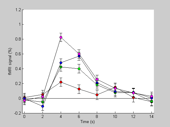
Example 4: Bootstrapping on residuals after regression: An fMRI example

'Event-related' fMRI involves a deconvolution between an fMRI time-series and an 'event sequence'. This is really a linear regression problem where the output is the predicted hemodynamic response.

This output are regressors, or values that when convolved with the event matrix predict the fMRI data with minimal least-squares error. The difference between the prediction and the actual data is called the residual.

We can obtain an estimate of the standard error for these regressors by bootsrapping on these residuals. That is, by repeatedly resampling the residuals with replacement and re-estimating the hemodynamic response. The standard deviation of these resampled estimates provides a measure of the standard error of our estimate.

This first part generates a fake hemodyamic response from an event-releated study with three event types (plus blank).

Experimental parameters

dt = 2;                 %step size, or TR (seconds)
maxt = 16;              %ending time for the estimated hdr (seconds)
th = 0:dt:(maxt-dt);    %time vector for plotting
n = length(th);         %length of the hdr.

Model parameters used for generating fake data

k = 1.25;           %seconds
nCascades = 3;
delay = 1;          %seconds

amps = [1,2,3,4];   %amplitudes of the hdr for the four event types (e.g. for increasing stimulus contrast).

true hdr are gamma functions with increasing amplitudes

h = zeros(n,4);
for i=1:4
    delay = 2; %seconds
    h(:,i) = amps(i)*gamma(nCascades,k,th-delay)';  %make it a column vector
end

Event sequence is an m-sequence

s = mseq(5,3);
m = length(s);
t = 0:dt:(m-1);

%Generate a concatenated design matrix
X = [];
for j=1:4
    Xj = zeros(m,n);
    temp = s==j;

    for i=1:n
        Xj(:,i) = temp;
        temp = [0;temp(1:end-1)];
    end
    X = [X,Xj];
end

%Predicted hemodynamic response (convolution of event matrix with hdr)
r = X*h(:);

%add IID noise
noiseSD = .25;
fMRI = r+noiseSD*randn(size(r));

Now for the interesting part. First we'll estimate the hdr from our data using linear regression (using the 'pinv' function).

hest = pinv(X)*fMRI;

Next we'll calculate the residual error between the model and the data

pred =X*hest;
resid = fMRI-pred;

Then we'll bootstrap by resampling the residuals, adding these new residuals to the prediction, and re-estimating the hdr. Note here that we're not calling the 'bootstrap' program but instead are just doing it manually. This because (1) we're not using the BCa method and (2) our 'statistic' has n values for each resample instead of just 1.

nReps = 1000;
sampHest = zeros(length(hest),nReps);
for i=1:nReps
    %resample residuals
    newResid = resid(ceil(rand(size(resid))*length(resid)));
    %generate new fMRI signal
    newFMRI = pred+newResid;
    %re-estimate the hdr
    sampHest(:,i) = pinv(X)*newFMRI;
end

The standard deviation of these re-estimated hdrs across resamples of the residual provides an estimate of the SEM for each time-point of the estimated hdr.

hestSEM = std(sampHest');

This part just reshapes the estimated hdr's into four columns - one for each event type (the original estimate comes out in one long vector).

hest = reshape(hest,n,4);
hestSEM = reshape(hestSEM,n,4);

Plot the estimated hdr's and their standard errors as error bars.

figure(1)
clf
hold on

colList = {'r','g','b','m'};
plot(th,zeros(size(th)),'k-');
for i=1:4
    errorbar(th,hest(:,i),hestSEM(:,i),'LineStyle','none','Color','k');
    plot(th,hest(:,i),'ko-','MarkerFaceColor',colList{i});
end
xlabel('Time (s)');
ylabel('fMRI signal (%)');
set(gca,'XLim',[-.25,max(th)+.25]);
set(gca,'XTick',th);

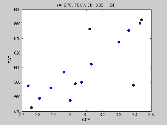
Example 5: Bootstrap on a correlation coefficient to get a confidence interval.

Bootstrapping on a correlation is useful because we know that the distribution of correlations is not normal since it's bounded between -1 and 1. Matlab provides an example data set of gpa and lsat scores for 15 students. We'll load it here and calculate the correlation.

load lawdata gpa lsat

sampStat = correlation([gpa,lsat]);

Show the scatter plot of GPA vs LSAT and display the correlation in the title.

figure(1)
clf
plot(gpa,lsat,'ko','MarkerFaceColor','b');
xlabel('GPA');
ylabel('LSAT');
title(sprintf('r = %5.2f,  %2.1f%% CI: [%5.2f, %5.2f]',sampStat,CIrange,CI(1),CI(2)));

Bootstrap the data by pulling out pairs with replacement. We'll use the 'BCa' method here.

nReps = 10000;
CIrange = 99;  %alpha <.01 (two-tailed)

[CI,sampStat,bootstrapStat] = bootstrap(@correlation,[gpa,lsat],nReps,CIrange);

Show the distribution of bootrapped values and the confidence interval

figure(2)
clf
xx = min(bootstrapStat):.01:max(bootstrapStat);
hist(bootstrapStat,xx);
hold on
ylim = get(gca,'YLim');
plot(sampStat*[1,1],ylim,'y-','LineWidth',2);
plot(CI(1)*[1,1],ylim,'r-','LineWidth',2);
plot(CI(2)*[1,1],ylim,'r-','LineWidth',2);
plot([1,1],ylim,'b-','LineWidth',2)
%set(gca,'XTick',[-10:.5:10]);
title('bootstrapping on a correlation coeficient');

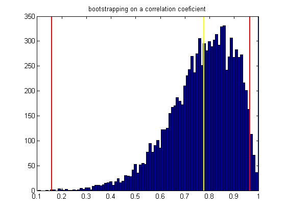
Since the lower end of our confidence interval is above zero, we conclude that our correlation is significant at the p<.01 level (two-tailed).

Example 6: Permutation test instead of bootstrapping

A 'permutation test' is a second resampling method that addresses the question of whether a correlation is significant or not. While the bootstrap method estimates a confidence interval around your measured statistic, the permutation test estimates the probability of obtaining your data by chance.

For the gpa lsat example, it involves shuffling the relationshiop between the two variables repeatedly and recalculating the correlation. It's like re-assigning one student's gpa with another student's lsat randomly to test the distribution of the null hypothesis that there is no relationship to the specific pairing of the two variables.

Computatinally, it is similar to the bootstrap method. On each iteration we'll shuffle the order of values in one of the variables before computing the correlation.

After many iterations, we'll compare the distribution of reshuffled correlations with our observed correlation. If it falls way out in the tail then we decide that we have a significant correlation.

Note, a true permutation test uses every possible reshuffling of the data. For our 15 observations, there are 15 factorial, or around a trillion combinations. To be reasonable, we'll just subsample 20,000 samples from these trillion combinations. This subsampling is called Monte Carlo simulation.

nReps = 100000;
perm = zeros(nReps,1);
for i=1:nReps
    %shuffle the lsat scores and recalculate the correlation
    perm(i) = correlation([gpa,shuffle(lsat)]);
end

determine how many reshuffled correlations exceed our observed value.

p = sum(perm>sampStat)/nReps;

Show a histogram of the reshuffled correlations and our observed value.

figure(1)
clf
hist(perm,50);
ylim = get(gca,'YLim');
hold on
plot(sampStat*[1,1],ylim,'r-','LineWidth',2);
xlabel('Correlation');
title(sprintf('Proportion of permutations exceending observed correlation: %5.5f',p));

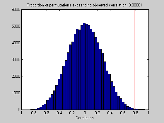
The standard statistical test for correlations is to assume a t-distribution with n-2 degrees of freedom. This test will conclude that we have a significant correlation with a p-value of 0.000665.

It is interesting to note the similarities and differences between the bootstrap and the permutation test here.

The bootstrap uses sampling without replacement while the permutation test samples with replacement (reshuffles).

The bootstrap preserves the pair-wise relationship between the two variables and therefore produces a distribution of values centered at our observed value. The permutation test does the opposite - shuffling the pairwise relationships and therefore produces a distribution centered at zero.

The decision in the bootstrap method is made by determining how much of the tail of the distribution falls below zero. The decision in the perumation test is made by determining how much of the distribution falls above our observed value.

I don't know which test is more appropriate, or whether they make similar decisions.

From Wikepedia:

Good (2000) explains the difference between permutation tests and bootstrap tests the following way: "Permutations test hypotheses concerning distributions; bootstraps tests hypotheses concerning parameters. As a result, the bootstrap entails less-stringent assumptions."

So there you go.

Good, P. (2002) Extensions of the concept of exchangeability and their applications, J. Modern Appl. Statist. Methods, 1:243-247.

Published with MATLAB® 7.6