Contents

Lesson 16: Auditory Motion

In this lesson, I'll introduce a simple method that converts a sound wave and a vector of x and y spatial position over time into a souund wave that simulates what an observer would hear while standing at the origin.

The method introduces the cues of interaural time delay (ITD) a doppler shift, and inverse square law. It also has a bit of an interaural level difference (ILD) because of the effect of the inverse square law and the fact that one ear will be closer to the sound than the other.

The trick is to calculate what the time-course of a sound wave should be at the location of the ear given the sound wave at the source, s(t), and the vectors of spatial position x(t) and y(t).

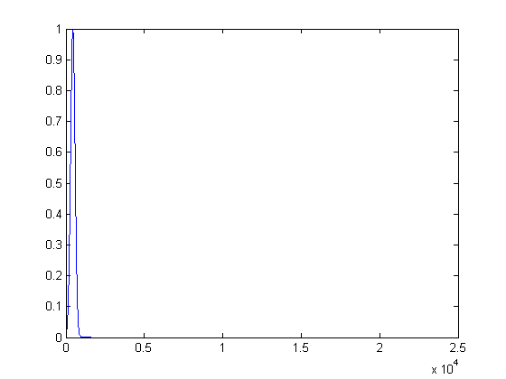
We'll start with a stationary band-pass sound. We'll then simulate what it should sound like when translating on a horizontal pass from left to right in front of your head. This first part should look familiar.

p.Fs = 44100;     % Sampling rate (Hz)
p.dur = 4;        % Duration (seconds)
centerFreq =440;  % Center of band-pass filter (Hz)
width = 200;      % Width of band-pass filter (Hz)

% Time vector
t= linspace(0,p.dur,p.dur*p.Fs)';

% White noise
y = randn(size(t));

% Fourier Transform:
F = complex2real(fft(y),t);

% Band-pass filter in the frequency domain:
Gaussian = exp(-(F.freq-centerFreq).^2/width^2)';
plot(F.freq,Gaussian);
F.amp = F.amp.*Gaussian;

% Inverse Fourier Transform:
s = real(ifft(real2complex(F)))';

% Play the sound
sound(s,p.Fs);

Auditory Horizontal Motion

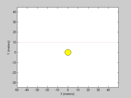
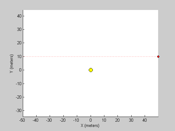
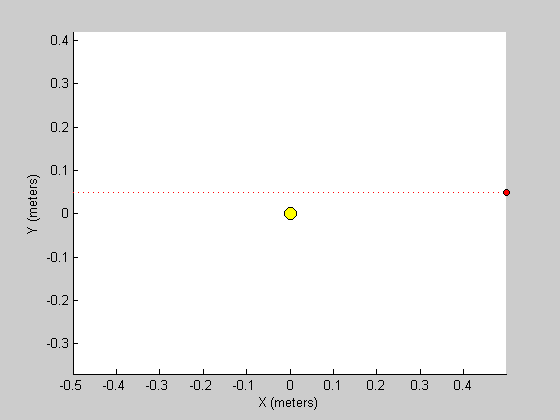
The next step is to set up vectors x and y that determine the location of the sound over time. The units will be in meters. This will be a sound traveling over the four seconds from 50 meters to the left to 50 meters to the right, 10 meters in front of you. (The speed of the sound source will therefore be a steady 25 meters/sec or about 56 mph). The graphics show a simple diagram of the position relative to your (yellow) head.

x = 50*linspace(-1,1,length(s))';
y = 10*ones(size(s));

figure(1)
clf
plot(x(1:200:end),y(1:200:end),'r:');
hold on
plot(0,0,'ko','MarkerSize',20,'MarkerFaceColor','y');
axis equal
xlabel('X (meters)');
ylabel('Y (meters)');

To calculate the sound at each of the two ears, we need to define the speed of sound and the width of the head:

p.c = 345;  %speed of sound (meters/second)
p.a = .0875;  %with of head (meters)

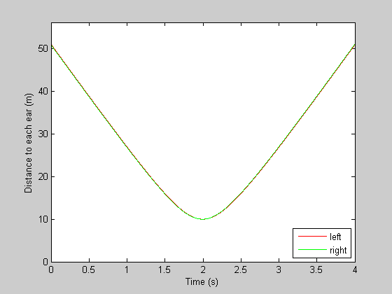
Next we'll calculate the distance (squared) from the source to each ear for each point in time. For illustration, we can plot these distances as a function of time.

dLsq = (x-p.a).^2+y.^2;
dRsq = (x+p.a).^2+y.^2;

figure(1)
clf
plot(t,sqrt(dLsq),'r-');
hold on
plot(t,sqrt(dRsq),'g-');
set(gca,'YLim',[0,sqrt(max(dLsq))*1.1]);
xlabel('Time (s)');
ylabel('Distance to each ear (m)');
legend({'left','right'},'Location','SouthEast');

Time delay to each ear

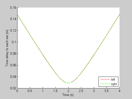
The sound received at each ear depends on how long it takes for the sound to travel from the source to each ear, as a function of time. The delay (tauL and tauR) is the distance to the ears divided by the speed of sound:

tauL = sqrt(dLsq)/p.c;
tauR = sqrt(dRsq)/p.c;

clf
hold on
plot(t,tauL,'r-');
plot(t,tauR,'g-');

xlabel('Time (s)');
ylabel('Time delay to each ear (m)');
legend({'left','right'},'Location','SouthEast');

Interaural Time Difference (ITD)

The Interaural Time Difference (ITD) is caused by the difference in distance of the object to the two ears. The time difference between the two ears will be the difference in the left and right distances divided by the speed of sound. Here's a plot of the ITD for our sound as a function of time:

ITD = 1000*(tauR-tauL);

clf
plot(t,ITD);
xlabel('Time (s)');
ylabel('ITD (msec)');

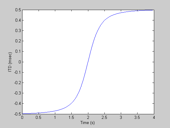
The ITD asymptotes at +/- 5 msec because it takes 5 msec for a sound to pass the width of the head. At the beginning and end of the sound, the position is pretty much on one side.

Inverse square law

The intensity of a sound drops of inversely with the square of the distance. We can simulate this by dividing our sound wave by our distance vectors. The two vectors are then combined to produce a two-channel (stereo) sound. There will be a very slight interaural level difference because one ear will always be closer to the sound than the other. But this is negligable for the distances here (as can seen by the overlap in the curves in the figure).

sL = s./dLsq;
sR = s./dRsq;

yy = [sL,sR];
yy = yy/max(yy(:));

sound(yy,p.Fs);

The Doppler effect

The Doppler effect is the change in pitch experienced by an observer as an object changes its speed relative to you. For illustration, we can plot the speed based on the rate of changes of the distances:

dt = 1/(t(2)-t(1));
speedL = diff(sqrt(dLsq))*dt;
speedR = diff(sqrt(dRsq))*dt;
clf
hold on
plot(t(1:end-1),speedL,'r-');
plot(t(1:end-1),speedR,'g-');

xlabel('Time (s)');
ylabel('Speed relative to each ear (m/s)');
legend({'left','right'},'Location','SouthEast');

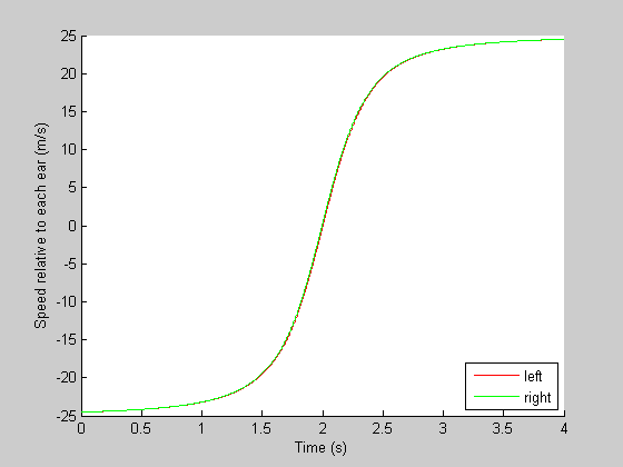
For the first half, the object is coming toward you at 25 m/sec(so the speed is negative). This will increase the pitch of the sound because the sound waves will effectively bunch up in front of the source. In the second half, as the object retreats, the pitch will be lower than the actual sound because the sound waves will be relatively spaced out behind the object.

Interpolating to simulate the sound at your head

Putting this all together might seem like a calculus nightmare. Fortunately it's really easy. All we need to do is re-sample the sound using linear interpolation based on our calculations of the time delay, after attenuating based on the inverse square law. The interpolation step uses 'interp1' which basically re-evaluates our sound wave with a different vector of time.

zero out the auditory stimulus matrix

yy = zeros(length(t),2);

Here's the interesting part: Interpolate back in time to determine sound for each ear and attenuate the sound based on inverse-square law

yy(:,1) = interp1(t,sL,t-tauR);
yy(:,2) = interp1(t,sR,t-tauL);

%clear out the NaN's (at the beginning of time where sound hasn't come to
%the head yet)
yy(isnan(yy))= 0;

yy = yy/max(yy(:));
sound(yy,p.Fs);

'makeAuditoryMotion.m'

I've provided a function 'makeAuditoryMotion' that performs the above calculations.

yy = makeAuditoryMotion(p,s,x,y);
yy = yy/max(yy(:));
sound(yy,p.Fs);

A cheesy animation

For fun, we can make a movie in the figure that moves our sound source over time while the sound is playing.

n= 1;  % number of times to loop.
figure(1)
clf

hold on

% Draw the 'Head'
plot(0,0,'ko','MarkerSize',10,'MarkerFaceColor','y');
axis equal

% Draw the path
plot(x(1:200:end),y(1:200:end),'r:');
h = plot(x(1),y(1),'ko','MarkerFaceColor','r','MarkerSize',5);
xlabel('X (meters)');
ylabel('Y (meters)');

%loop n times

for i=1:n
    %play the sound
    sound(yy,p.Fs);
    %animate the object
    tic
    while toc<p.dur
        %Find index that matches closest to the current time
        id = ceil(toc*p.Fs);
        set(h,'XData',x(id));
        set(h,'Ydata',y(id));
        drawnow
    end
end

animateAuditoryMotion

I've also provided a function 'animateAuditoryMotion' that runs 'makeAuditoryMotion' and plays it along with our cheesy animation. It's essentially the same code as above.

animateAuditoryMotion(p,s,x,y,2);

Recording a sound

Matlab's function 'audiorecorder' allows you to record your own sounds with a built-in microphone or an external one. It's easy to use. Here we'll sample a little over 4 seconds of sound and clip it so it's exactly four seconds so that it's compatible with our existing x and y vectors.

r = audiorecorder(p.Fs, 16, 1);

record(r);     % speak into microphone...
pause(4.2)
stop(r);

s =  getaudiodata(r);
s = s(1:length(t));

sound(s,p.Fs);   % listen to complete recording

Now we'll make it move!

animateAuditoryMotion(p,s,x,y,2);

Other sounds, other paths

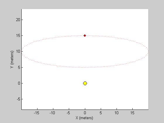
Since this is all done with simulation and not with calculus, we can simulate any sound with any path. Here are some examples:

load handel
s = y;
p.Fs = Fs;
p.dur = length(s)/p.Fs;  %duration of sound (second)

t= linspace(0,p.dur,length(s))';

%position of sound over time (in meters, with observer at [0,0])
x = 20*sin(2*pi*t/p.dur);
y = 5*cos(2*pi*t/p.dur)+10;

%translate sound wave and position into stereo sound wave
[yy,p] = animateAuditoryMotion(p,s,x,y,1);

p.dur = 4;
p.Fs = 44100;

t= linspace(0,p.dur,p.dur*p.Fs)';
s = floor(rand(size(t))+.001);

x = linspace(-.5,.5,length(t))';
y = .05*ones(size(t));

[yy,p] = animateAuditoryMotion(p,s,x,y,1);

Exercises

1) Combining sounds is easy. Just add two sound waves together - but be sure that the sum stays between -1 and 1. Generate the sound of low frequency moving from left to right and high frequency moving from right to left. Can you attentively separate the two sounds? What if they are the same frequency?

2) A sonic boom occurs when a noisy object moves at the speed of sound, where the sound waves all pile up in front of the object. Can you simulate a sonic boom?

3) What happens to a sound that is receeding from you faster than the speed of sound?

Published with MATLAB® 7.6