Lesson 17: Independent Components Analysis

Supose you have two microphones (or two ears) in two places in a room, and each is recording the sound produced by two sources in two other places in the room. To a first approximation, the sound entering each microphone will be a linear combination of each of the two sound sources, weighted differently depending on how far away each microphone is away from each source. 'Independent Component Analysis', or ICA is a way to unmix these two recordings to estimate the two original separate sound sources. ICA generalizes to higher dimensions so that you should be able to separate three sources given at least three recordings, and so on. This lesson will focus on the 2-D case for simplicity.

Contents

Assumptions

For ICA to work perfectly, three things have to be true:

1) Each measured signal is a linear combination of the sources (like the sound example above)

2) The sources need to be uncorrelated

3) The histograms for each source cannot be Gaussian (this may seem strange, but you'll see why later)

ICA falls apart as these assumptions become less true, but still works remarkably well for minor violations.

We'll demonstrate how ICA works by taking two uncorrelated, non-Gaussian signals and combining them linearly to make two new measured signals. Then we'll go through the steps for ICA to 'undo' the linear combinations to get our original two sources back. We can think of the sources and signals in the context of the sound example above.

Two sources

First, we'll set up a time vector and generate the two sources (as column vectors): One will be a sinusoid and the other will be uniformly distributed noise. You can think of one as signal and the other as noise:

t = linspace(0,1,500)';
y1 = sin(6*pi*t);
y2 = rand(size(t));

It makes things simpler if our measured sources have zero mean and a standard deviation of 1:

y1 = (y1-mean(y1))/std(y1);
y2 = (y2-mean(y2))/std(y2);

Here's a graph of the two sources:

figure(1)
clf
subplot(2,1,1)
plot(t,[y1,y2]);

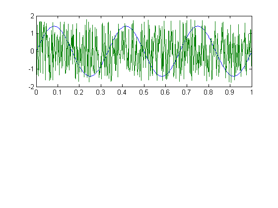
We've actually already violated one of the two assumptions - the correlation between these two vectors won't be exactly zero (it has an expected value of zero, but each example will be off by some random amount). If you squint, you might see this in a scatter plot comparing y1 to y2:

subplot(2,1,2)
plot(y1,y2,'.');

axis equal
axis tight

Here's the correlation:

disp(correlation(y1,y2));

    0.0212

This slight correlation means that we won't get our exact sources back. But we'll be close.

Combining the two sources

Suppose the first of our two measured time-courses is made up of 80% of y1 and 50% of y2 (they don't have to add up to 100%). And suppose the second recording is 10% y1 and 40% y2. We can use matrix multiplication using the 'weight matrix':

A = [.8,.5 ; .1,.4]

A =

    0.8000    0.5000
    0.1000    0.4000

and let:

X = [y1,y2]*A;

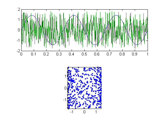
If you remember how matrix multiplication works, then you'll see that each column of X is a linear combination of y1 and y2 with the weights specified by A. The two columns of X will be our 'mixed' time-series. We can plot these time-series and the corresponding scatter plot in figure 2, like we did in figure 1:

figure(2)
clf
subplot(2,1,1)
plot(X)
subplot(2,1,2)
plot(X(:,1),X(:,2),'.')
axis equal
axis tight

The two measured time-courses each look like sinusoids with noise added, which is exactly what they are. Each microphone is picking up some signal and some noise. They're strongly correlated with each other, as can be seen in the scatter plot. Let's look at their correlations:

disp(correlation(X(:,1),X(:,2)))

    0.8565

Decorrelating or 'whitening' the signals

ICA unmixes the linear combinations by taking advantage of the three assumptions above, step by step. The first assumption, that our measurements are linear combinations of the sources, means that it should be possible to 'undo' the linear combination with another linear combination. Actually since we made up our own data, we can easily undo things by multiplying X by the inverse of our mixing matrix A:

Y = X*inv(A);

Of course, in the real world we don't know how these two sources were combined, so we have to find this 'unmixing' matrix ourselves.

The first step is to take advantage of assumption 2, which is that the sources are uncorrelated.

We need to find a new 2x2 matrix, W, so that when multiplied by X will give us two uncorrelated vectors. Even more, we want the variance of each vector to be equal to one.

An equivalent way to say this is that we want the covariance of X*W to be equal to the identity matrix. This takes a little linear algebra, but

In the example here with matrices, I have a matrix X and a mixing matrix W, and I want to find the matrix W so that cov(X*W) = I. It turns out that you can find W by finding the matrix equivalent of 1/sqrt(cov(X)):

W= inv(sqrtm(cov(X)));

This decorrelating process is sometimes called 'whitening' because it produces two uncorrelated signals with unit variance, which is the definition of white noise.

Xwhite = X*W;

Check the covariance for ourselves:

cov(X)
cov(Xwhite)

ans =

    0.6534    0.4478
    0.4478    0.4185


ans =

    1.0000    0.0000
    0.0000    1.0000

cov(Xwhite) is the identity matrix. This means that the two columns each have a variance of 1, and the correlation of the two columns is equal to zero, as desired.

The whitening process is a standard trick in linear algebra, but to understand it requires some knowledge of the algebra of covariance matrices and eigenvectors.

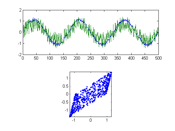
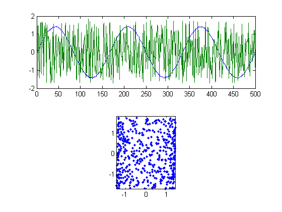
By now you might be confused. It'll help to look at a picture of our new vectors in Xwhite:

figure(3)
clf
subplot(2,1,1)
plot(Xwhite)
subplot(2,1,2)
plot(Xwhite(:,1),Xwhite(:,2),'.')
axis equal
axis tight

Rotating the scatterplot

Our two new vectors shown in figure 3 are a step closer to unmixing the original signals. They satisfy the assumption of independence. But we're not quite there yet. Compare the scatterplots in figure 3 to figure 1. It should be that we need to rotate the scatterplot in Figure 3.

This is because there are a whole family of matrices that can 'whiten' the matrix X. The linear algebra trick above (W = inv(sqrtm(cov(X))) gives just one of them. Matrices that produce any rotation of the scatterplot is also a whitening matrix.

To rotate the scatterplot in figure 3 can be done with yet another matrix multiplication. This time by a 2x2 'rotation matrix', R.

It looks like we want to rotate the scatterplot in figure 3 clockwise by 5 degrees or so, or 5*pi/180 radians. This can be done by multiplying Xwhite by this matrix:

ang = -5*pi/180;
R = [cos(ang), sin(ang); - sin(ang) cos(ang)];

Xwhiterot = Xwhite*R;

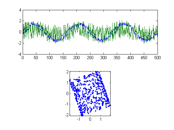
We can view our newest signals as we've done in the previous figures:

figure(4)
clf
subplot(2,1,1)
plot(Xwhiterot)
subplot(2,1,2)
plot(Xwhiterot(:,1),Xwhiterot(:,2),'.')
axis equal
axis tight

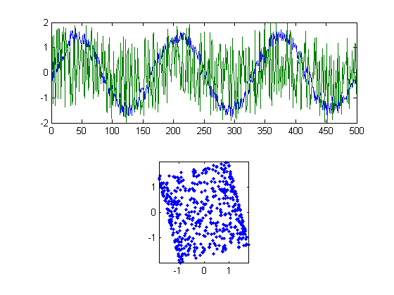
Our rotation matrix actually rotates things clockwise by 'ang', which why we set ang to be -5.

We're almost there! The two signals in figure 4 look a lot like the original sources in figure 1. It just looks like we're off by just a little bit of rotation.

Rotating to maximize kurtosis

Our value of -5 degrees was just a guess. We now use an objective method to find the best angle to rotate the two signals to get our original sources back. This is done by taking into account our third assumption - that our original sources do not have Gaussian histograms.

This is the real clever bit. Remember the Central Limit Theorem? Probably not. It says that the sum (or mean) of two random samples will tend to be more normally distributed than the original samples. Recall that a rotation is just a linear combination of the two columns. Since our original signals were non-Gaussian, and Xwhite is a linear combination of our original signals, it follows that the columns of Xwhite should be more normally distributed than than or original signals. The trick is to rotate Xwhite so that the columns are as non-normal as possible. This will be the rotation that gives us our best estimate of the original signals.

There are a variety of measures of non-normality that are used in ICA algorithms. The simplest is kurtosis, which measures the heaviness of the tails in a distribution. A normal distribution will have a kurtosis of 3. Skinnier distributions will have a kurtosis less than 3, broader greater than 3.

I've provided a function 'kurtMat' that calculates the kurtosis of each column of a matrix and returns the norm of these values (square root of sum of squares). This gives us the single measure of normality for our two signals that we need to minimize. For example, the kurtosis of our original two signals is:

kurtMat([y1,y2])

ans =

    2.3668

The kurtosis of our measured signals is

kurtMat(X)

ans =

    2.7548

There's the Central Limit at Theorem at work: the columns of X are linear combinations of y1 and y2 and therefore more normally distributed.

Our whitened, rotated data, Xwhiterot should have a kurtosis similar to our original signals y1 and y2:

kurtMat(Xwhiterot)

ans =

    2.5924

Let's find the rotation angle that gives us the kurtosis that's furthest from 3. We'll use our 'fit' program to do a brute-force search. This will require a function that takes in a rotation parameter as a field of a structure and our whitened signals, and returns an error value to be minimized. Here's the process:

p.ang = -10*pi/180;

R = [cos(p.ang), sin(p.ang) ; -sin(p.ang) cos(p.ang)];
Xwhiterot = Xwhite*R;
err = -abs(kurtMat(Xwhiterot)-3);

The values of err will be negative. The more the kurtosis differs from 3, the more negative err will be. I've put this code into the function 'kurtMatErr'. Here's how to use it:

err= kurtMatErr(p,Xwhite)

err =

   -0.5307

It's ready for the 'fit' routine which will find the value of p.ang that minimizes 'err':

pBest = fit('kurtMatErr',p,{'ang'},Xwhite);

Fitting "kurtMatErr" with 1 free parameters.

The best rotation angle in degrees is:

disp(pBest.ang*180/pi)

  -20.0039

kurtMatErr also returns our optimal signals as a second argument and the corresponding rotation matrix as the third argument. Let's get them:

[err,Xwhiterotbest,Rbest] = kurtMatErr(pBest,Xwhite);

'Xwhiterotebest' should be our best guess at the optimal rotation, which should give us our best estimate of the original signals [y1,y2] that we used get 'X'. We'll plot the results in figure 5.

figure(5)
clf
subplot(2,1,1)
plot(Xwhiterotbest)
subplot(2,1,2)
plot(Xwhiterotbest(:,1),Xwhiterotbest(:,2),'.')
axis equal
axis tight

Not bad. We've used our three assumptions to get back the two signals that we mixed together for the matrix X. The kurtosis of our best estimate should be close to our original signals too:

kurtmat([y1,y2])
kurtMat(Xwhiterotbest)

Warning: Could not find an exact (case-sensitive) match for 'kurtmat'.
C:\Users\Geoff
Boynton\Documents\courses\Matlab_2_S12\web\matlab\kurtMat.m is a
case-insensitive match and will be used instead.
You can improve the performance of your code by using exact
name matches and we therefore recommend that you update your
usage accordingly. Alternatively, you can disable this warning using
warning('off','MATLAB:dispatcher:InexactCaseMatch').
This warning will become an error in future releases. 

ans =

    2.3668


ans =

    2.3612

Sometimes you'll get your two components back, but switched. ICA is 'blind' to the original sources, so it doesn't 'know' which signal to call y1 and which to call y2.

Also, since our estimated sources are required to have a mean of zero and a variance of 1, they will necessarily differ from the original by a scale factor. In our example, y1 and y2 are already normalized so that's not an issue here.

Putting it all together

Our goal was to find a single 2x2 matrix that unmixes our two measures signals into two uncorrelated, or 'independent' sources. The code above incorporated two steps, whitening rotating. These two steps each had an associated mixing matrix. For whitening it was W= inv(sqrtm(cov(X))). For rotating it is the rotation matrix associated with pBest.ang, Rbest.

Given these two matrices, the whole process can be done in one line:

Xwhiterotbest = (X*W)*Rbest;

Any two successive matrix multiplications can be summarized as a single matrix multiplication. That's because matrix multiplication is associative:

Xwhiterotbest = X*(W*Rbest);

so our complete ICA mixing matrix is:

M = W*Rbest;

The inverse of this matrix is very useful. While M tells you how to get from our measured signals back to the original sources, the inverse of M goes the other way - it tells you how to get from the sources to your measured signal. If all works well, then for our example, the inverse of M should be very close to the actual matrix that we used to mix our sources, A

A
inv(M)

A =

    0.8000    0.5000
    0.1000    0.4000


ans =

    0.8041    0.5170
    0.0827    0.3889

Comparing A and inv(M) gives us our best estimate for how well the ICA algorithm is working, since A is our actual mixing matrix. But if we didn't have A (like in real life), inv(M) is very useful for predicting what a given measured signal should be given any possible source.

Unmixing two real sounds

Load in the sounds and place them into a single matrix Y

s1 = load('splat');
s2 = load('train');

n = max(length(s1.y),length(s2.y));

Y = zeros(n,2);
Y(1:length(s1.y),1) = s1.y;
Y(1:length(s2.y),2) = s2.y;

Y = (Y-repmat(mean(Y),n,1))./repmat(std(Y),n,1);

Mix the sounds with a mixing matrix

A = [.3,.7;.8,.2];
X = Y*A;

soundsc(X(:,1))
soundsc(X(:,2))

Unmix using the same steps as above

Xwhite = X*inv(sqrtm(cov(X)));
p.ang = 0;
pBest = fit('kurtMatErr',p,{'ang'},Xwhite);
[err,Xunmixed,Rbest] = kurtMatErr(pBest,Xwhite);

soundsc(Xunmixed(:,1))
soundsc(Xunmixed(:,2))

Fitting "kurtMatErr" with 1 free parameters.

How it's acutally done

There are a varity of ICA algorithms that vary by their measures of 'normality' for optimally rotating the matrix. Kurtosis is easy and intuitive, but it's also sensitive to outliers. Other routines use ideas from information theory to avoid this problem. We won't go into that here because the general intuition is the same.

Other routines don't use matlab's nonlinear parameter estimation program like we did to find the best rotation. Instead they use some tricks like 'fixed-point' algorithms which are much more efficient. But again, the intuition is the same. I don't recommend you use this algorithm here if you really want to use ICA - this should really only serve as a tutorial. Besides, it only works for two dimensions.

There are a bunch of Matlab ICA implementations out there. One I find that's fast and works well is 'fastica', which can be obtained from a group at the Helsinki University of Technology:

http://research.ics.tkk.fi/ica/fastica/

Exercises

Published with MATLAB® 7.11