Lesson 18: Diffusion or random walk models of reaction times

This lesson covers the most basic model for predicting the frequency distributions and accuracy in a reaction time (RT) experiment, the random walk or diffusion model. I learned much of this from a very accessible paper by Palmer, Huk and Shadlen:

Palmer, Huk & Shadlen (2008) Journal of Vision http://www.journalofvision.org/5/5/1/

Contents

What is a 'diffusion process'?

The basic idea is that decisions are made by accumulating information over time. Specifically, evidence is represented as a variable that increments or decrements over time based on incoming information. I can't summarize it better than Palmer, Huk and Shadlen:

"The internal representation of the relevant stimulus is assumed to be noisy and to vary over time. Each decision is based on repeated sampling of this representation and comparing some function of these samples to a criterion. For example, suppose samples of the noisy signal are taken at discrete times and are added together to represent the evidence accumulated over time. This accumulated evidence is compared to an upper and lower bound. Upon reaching one of these bounds, the appropriate response is initiated. If such a random walk model is modified by reducing the time steps and evidence increments to infinitesimals, then the model in continuous time is called a diffusion model (Ratcliff, 1978; Smith, 1990). For this model, the accumulated evidence has a Gaussian distribution, which makes it a natural generalization of the Gaussian version of signal detection theory (Ratcliff, 1980)." (Diffusion processes are also known as the Wiener process or Brownian motion)

Intuitively, you can imagine how this simple model can predict error rates, and RTs for both correct and incorrect responses. In the simplest case, analytical solutions exist for accuracy and the distribution of RTs.

This lesson simulates a simple random walk model, calculating accuracy and histograms of RTs. The results of the simulation is then compared to curves generated from the analytic solution.

Define variables for the random walk:

The basic random walk model consists of a variable that increments or decrements over time until a criterion value is reached. The units of this variable are arbitrary - they could all vary by a scale factor together without any effect on the model. The parameters of the model consist of upper and lower bounds for stopping the walk to make a decision, a mean drift rate or bias (upward or downward), and a standard deviation of the drift, which the source of noise or variability.

p.a = .15;  %upper bound (correct answer)
p.b = .1;   %lower bound (incorrect answer)
p.s = .1;   %standard deviation of drift (units/sec)
p.u = .075; %drift rate (units/sec)

p.dt = .1;  %step size for simulations (seconds)

First let's do a quick simulation of the random walk model without worrying about keeping track of RTs.

nReps = 5; %number of staircases per simulation
nSteps = 30; %number of time steps

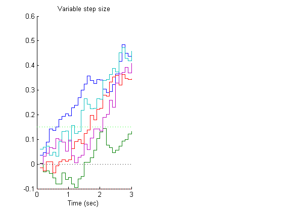
Random walk with variable step sizes

One way to simulate a biased random walk is to have step sizes pulled from a normal distribution with mean u*dt and standard deviation s*sqrt(dt). Why sqrt(dt)? Because variance adds linearly over time, so standard deviation adds by sqrt(dt). This way, after 1 second, the distribution of walks should be distributed with a mean of p.u and a standard deviation of p.s. What do you think the mean and standard deviation will be after two seconds?

dy = p.u*p.dt + p.s*sqrt(p.dt)*randn(nSteps,nReps);

%The random walk is a cumulative sum of the steps (dy)
y = cumsum(dy);

%plot it.

t = p.dt:p.dt:p.dt*nSteps; %time vector for x-axis
figure(1)
clf
subplot(1,2,1)
hold on

%plot the bounds
plot([0,p.dt*nSteps],[0,0],'k:');
plot([0,p.dt*nSteps],[p.a,p.a],'g:');
plot([0,p.dt*nSteps],-[p.b,p.b],'r:');


stairs(t,y);
xlabel('Time (sec)');
title('Variable step size');

Fixed step size with biased coin

A second way to implement the diffusion model is to fix the step sizes and flip a biased coin to determine whether the walk goes up or down.

The up and down step size is s*sqrt(dt) - same as the standard deviation of the step size above.

yStep = sqrt(p.dt)*p.s;

The coin is biased by the drift rate. Let's derive it. If p is the probability of going up, then the expected dy of a given step is yStep*p - yStep*(1-p) = yStep*(2p-1) = s*sqrt(dt)*(2p-1). This should be equal to the drift rate, u*dt. So s*sqrt(dt)*(2p-1) = u*dt. Solving for p (prob) gives:

prob = .5*(sqrt(p.dt)*p.u/p.s + 1);

%To implement this, use the 'rand' and 'sign' functions:

dy = yStep*sign(rand(nSteps,nReps)-(1-prob));
y = cumsum(dy);

plot it

subplot(1,2,2)
hold on

%plot the bounds
plot([0,p.dt*nSteps],[0,0],'k:'); %zero
plot([0,p.dt*nSteps],[p.a,p.a],'g:'); %upper bound (correct responses)
plot([0,p.dt*nSteps],-[p.b,p.b],'r:');%lowe bound (incorrect responses)

stairs(t,y);
xlabel('RT (s)');
title('Coin flip');

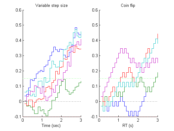
Like before, the distribution of values after 1 second should have a mean of p.u and a standard deviation of p.s.

Simulating RT distributions

The walk should stop when the acculating variable hits one of the decision bounds. The time step when this happens is the RT for that trial.

We'll implement this with a loop over time. We'll only keep track of the current values of y, and only increment the walks that haven't lead to a decision.

nReps = 1000;  %number of simulated walks
p.dt = 1/1000; %time step (seconds)

%Initalize some parameters:

alive = true(1,nReps);      %index vector for walks that haven't terminated
y = zeros(1,nReps);         %current position for each walk (starting at 0)
response = zeros(1,nReps);  %to be filled with -1 or 1 for incorrect and correct
RT = zeros(1,nReps);        %to be filled with RT values in seconds

For the coin-flip random walk, as before:

yStep = sqrt(p.dt)*p.s;
prob = .5*(sqrt(p.dt)*p.u/p.s + 1);

tStep = 0;
while sum(alive) %loop until all walks are terminated
    tStep = tStep+1;

    %for continuous step sizes, use this line:
    %dy = p.u*p.dt + p.s*sqrt(p.dt)*randn(1,sum(alive));

    %for 'coin flip' steps, use this line:
    dy =  yStep*sign(prob-rand(1,sum(alive)));

    %increment the 'living' walks
    y(alive) = y(alive)+ dy;

    %find the walks that reached a correct decision:  the 'a' boundary
    aboveA = find(y>=p.a & alive);
    if ~isempty(aboveA)
        response(aboveA) = 1; %correct response
        alive(aboveA) = false; %'kill' the walk
        RT(aboveA) = tStep*p.dt; %record the RT
    end
    %find the walks that reached an incorrect decision: the '-b' boundary
    belowB = find(y<=-p.b & alive);
    if ~isempty(belowB)
        response(belowB) = -1;  %incorrect response
        alive(belowB) = false; %'kill' the walk
        RT(belowB) = tStep*p.dt; %record the RT
    end
end

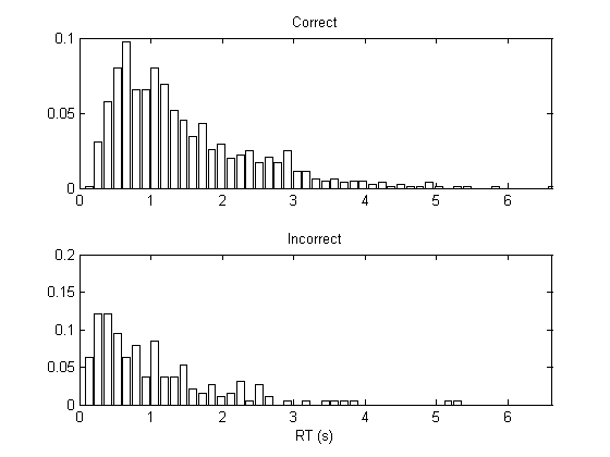
Plot histograms of simulated RTs

bins = linspace(0,max(RT),51); %Set time bins for histograms

figure(2)
clf
subplot(2,1,1) %correct
n=hist(RT(response==1),bins);
n = n/sum(response==1);
%stairs(bins,n,'b-','LineWidth',2);
bar(bins,n,'w');

set(gca,'XLim',[min(bins),max(bins)]);
title('Correct');

subplot(2,1,2) %incorrect
n=hist(RT(response==-1),bins);
n = n/sum(response==-1);
bar(bins,n,'w')
set(gca,'XLim',[min(bins),max(bins)]);

xlabel('RT (s)');
title('Incorrect');

Analytical solution to the diffusion model

It turns out that for the diffusion model there is an analytical solution to predict the percent correct and the frequency distribution of RTs (including the mean). Some smart people like Roger Ratcliff (1978) and Duncan Luce have worked this out using some interesting math that is beyond the scope of this lesson. For more information on this see Luce's 1986 book 'Response times' and the JOV paper mentioned above.

I've provided some functions that provide these solutions given our paramter values:

help expectedPC

 PC = expectedPC(p)
 
 expected probability correct for the standard diffusion model
 
 Inputs:
  p.a  upper bound (correct answer)
  p.b  lower bound (incorrect answer)
  p.s  standard deviation of drift (units/sec)
  p.u  drift rate (units/sec)

help expectedRTpdf

  pdfRT = expectedRTpdf(p,[t],[kRange])
 
  Calculates the analytical solution for the distrubution RT's on correct
  trials for a diffusion model with the following parameters (as fields in
  the structure 'p'):
 
  p.a  upper bound (correct answer)
  p.b  lower bound (incorrect answer)
  p.s  standard deviation of drift (units/sec)
  p.u  drift rate (units/sec)
 
  required function: expectedPC.m

help expectedMeanRT

  meanRT = expectedRTpdf(p)
 
  Calculates the analytical solution for mean RT for correct and incorrect
  trials for a diffusion model with the following parameters (as fields in
  the structure 'p'):
 
  p.a  upper bound (correct answer)
  p.b  lower bound (incorrect answer)
  p.s  standard deviation of drift (units/sec)
  p.u  drift rate (units/sec)

Let's compare the simulated accuracy to the analytical solution.

Call the function 'expectedPC' which gives the expected probability correct.

PCsimulation = sum(response==1)/nReps;
PCmodel = expectedPC(p);

disp(sprintf('simulated PC: %%%5.2f, model PC: %%%5.2f',PCmodel*100,PCsimulation*100));

simulated PC: %79.56, model PC: %81.10

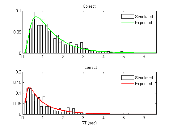
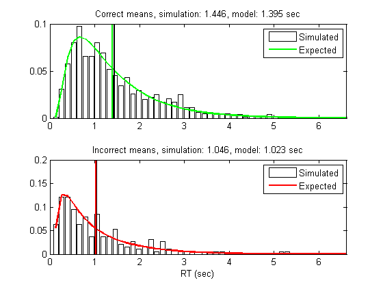
Compare the distribution of the simulated RTs to the analytical solution.

Call the function 'expectedRTpdf' which gives the expected pdf (histograms) of the RTs for correct answers.

[pdfRTcorrect,pdfRTincorrect] = expectedRTpdf(p,bins);  %scale by time step (dt)

pdfRTcorrect = pdfRTcorrect*(bins(2)-bins(1));
pdfRTincorrect=pdfRTincorrect*(bins(2)-bins(1));

Draw the analytical solution on top.

subplot(2,1,1)
hold on
plot(bins,pdfRTcorrect,'g-','LineWidth',2);
legend({'Simulated','Expected'});

subplot(2,1,2)
hold on
plot(bins,pdfRTincorrect,'r-','LineWidth',2);
legend({'Simulated','Expected'});
xlabel('RT (sec)');

Plot the real and predicted mean RT's

[meanRTcorrect,meanRTincorrect] = expectedMeanRT(p);

subplot(2,1,1)
ylim = get(gca,'YLim');
plot(mean(RT(response==1))*[1,1],ylim,'k-','LineWidth',2);
plot(meanRTcorrect*[1,1],ylim,'g-','LineWidth',2);
title(sprintf('Correct means, simulation: %5.3f, model: %5.3f sec',mean(RT(response==1)),meanRTcorrect));

subplot(2,1,2)
ylim = get(gca,'YLim');
plot(mean(RT(response==-1))*[1,1],ylim,'k-','LineWidth',2);
plot(meanRTincorrect*[1,1],ylim,'r-','LineWidth',2);
title(sprintf('Incorrect means, simulation: %5.3f, model: %5.3f sec',mean(RT(response==-1)),meanRTincorrect));

Exercises

Published with MATLAB® 7.11