Contents

Lesson 20: Pattern Classification Tutorial

randn('seed',0);

In this tutorial we'll work through some of the basic classification methods used in computer science, leading up to how it can be used to classify stimuli in a 'multivoxel pattern classification' experiment.

How can you tell a dog from a cat? A small child can do this easily, but if you think about it it's actually a difficult problem. Presumably we take into account various features of an animal and compare it to what we already know about categories that we've learned over our lifetime. For example, features that distinguish cats from dogs might be the shape of the eyes, shapes of the ears, length of the nose, or perhaps the ratio between various features like tail and leg length. Often values along any one dimension will overlap between categories so we somehow have to integrate information across all relevant dimensions to make a decision.

A lot of research has gone into how people learn to classify things. It's something we're really good at - it's a fundamental skill that allows us to not only categorize objects, but also recognize letters, understand speech, and guess the mood of your spouse.

A lot of research has also gone into getting computers to classify things. Like a lot of topics in computer science, this work has evolved in parallel with human research. Computer algorithms can now classify images and recognize speech with an ability that rivals humans. The 'machine learning' algorithms that do this are complex, but it it all started with a simple algorithm called 'discriminant analysis classification', which is the topic of this Tutorial.

As with many of the other tutorials in this class, we'll generate fake data under known statistical conditions, and see how well we can reconstruct our data using these algorithms.

One class and two dimensions: Cats eyes and noses

Before we get started on classification, we first need to define what we mean by 'class'. In discriminant analysis, a 'class' is defined as a set of items that have a set of features drawn from some probability distribution. Let's take a concrete example: cats. Cats have oval shaped eyes and short noses. Using aspect ratio as our dimension for eyes, let's assume that the population of cats have a mean eye-shape of 2, with a standard deviation of 1. Using an arbitrary of nose length, let's assume that nose lengths have a mean of 1 with a standard deviation of 1.

Bivariate normal distributions

The simplest discriminant analysis methods assume that the probability distributions for our features are normally distributed. For our cats, which are defined with two features, their features are distributed with a 'bivariate normal' probability distribution.

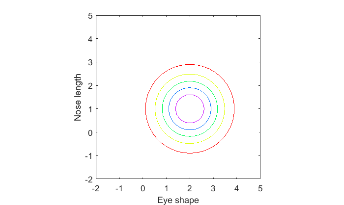
The simplest bivariate normal distribution has no correlation between the features. Let's assume this for our cats. This means that knowing a cat's eye-shape won't tell you anything about that cat's nose length.

Let's also assume that the distribution of eye-shape and nose length have equal variance.

We can visualize this bivariate probability distribution function as a surface in two-dimensions. Matlab's 'mvnpdf' gives you the probability distribution for a bivariate (or multivariate) normal distribution.

[xx,yy] = meshgrid(linspace(-2,5,301));

m1 = [2,1];  %  means for cats: eye shape = 2, nose length = 1

X = [xx(:),yy(:)];  %Turn grids xx and yy into a matrix with two columns.
p1 = mvnpdf(X,m1);
p1 = reshape(p1,size(xx));  %turn the output back into the shape of the grid.

figure(1)
clf
surf(xx(1,:),yy(:,1),p1,'LineStyle','None');
xlabel('Eye shape')
ylabel('Nose length');
view([-30,35])

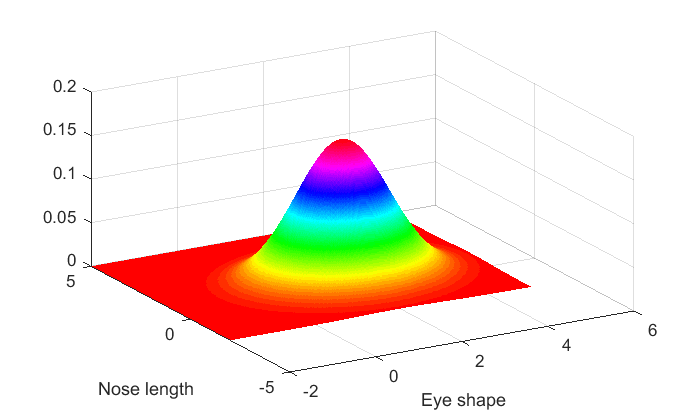
A contour plot might be more insightful. An uncorrelated bivariate normal distribution has circular contour lines:

cLevels = linspace(0,1,7)*max(p1(:));

figure(1)
clf
contour(xx(1,:),yy(:,1),p1,cLevels);
xlabel('Eye shape')
ylabel('Nose length');
axis equal

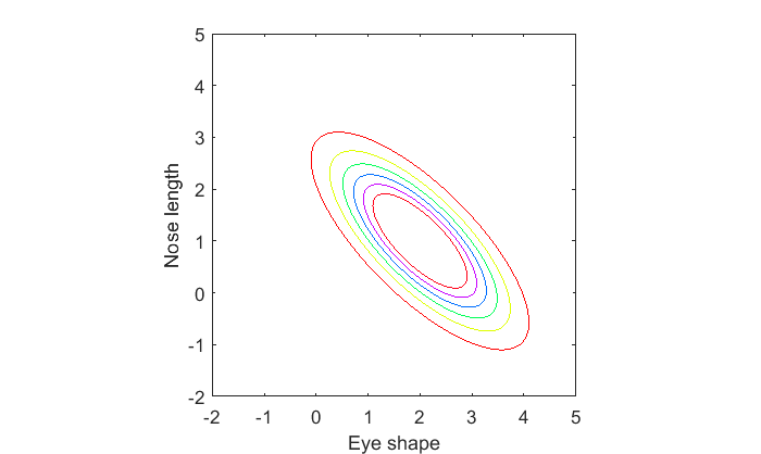
Suppose that there is a relation between eye-shape and nose length. Let's say that cats with more oval eyes have shorter noses (I'm making this up of course). In this case, eye-shape and nose length 'covary'. The way they covary can be defined with a covariance matrix, which is a 2x2 symmetric matrix where the diagonals are the variances for each dimension, and the off-diagonal is the covariance between the two variables.

For a really nice tutorial on the geometric interpretation of the covariance matrix, see:

http://www.visiondummy.com/2014/04/geometric-interpretation-covariance-matrix/

We'll set the covariance to a value of -.75. You can see how the features of eye-shape and nose length are anti-correlated:

S1 = [1,-.75;
    -.75,1];

p1 = mvnpdf(X,m1,S1);
p1 = reshape(p1,size(xx));

figure(1)
clf
contour(xx(1,:),yy(:,1),p1,cLevels);
xlabel('Eye shape')
ylabel('Nose length');
axis equal

Two classes and two dimensions: Cats and Dogs, Eyes and Noses

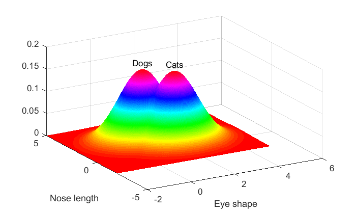
Now let's consider a second class of animal, dogs. Dogs typically have round eyes and cats have oval-shaped eyes. Let's assume that dog's eyes have a mean aspect ratio of 1 compared to the cat's mean aspect ratio of 2.

Dogs usually have longer noses than cats. Let's assume that dogs have noses with a mean length of 2 compared to the cat's mean length of 1.

We'll go back to the case where the dimensions are uncorrelated and take a look at the two probability distributions:

% cats:
m2 = [2,1];  %  means for cats: eye shape = 2, nose length = 1

p1 = mvnpdf(X,m1);
p1 = reshape(p1,size(xx));

% dogs:
m2 = [1,2];  %  means for cats: eye shape = 2, nose length = 1

p2 = mvnpdf(X,m2);
p2 = reshape(p2,size(xx));

figure(1)
clf
surf(xx(1,:),yy(:,1),p1,'LineStyle','none');

text(m1(1),m1(2),max(p1(:))*1.1,'Cats','HorizontalAlignment','center');
hold on

surf(xx(1,:),yy(:,1),p2,'LineStyle','none');
text(m2(1),m2(2),max(p2(:))*1.1,'Dogs','HorizontalAlignment','center');

xlabel('Eye shape')
ylabel('Nose length');
view([-30,35])

Or as contour plots:

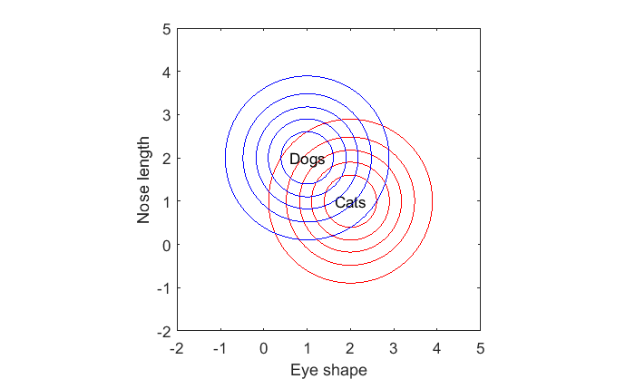
figure(1)
clf
contour(xx(1,:),yy(:,1),p1,cLevels,'Color','r');

text(m1(1),m1(2),'Cats','HorizontalAlignment','center');
hold on

contour(xx(1,:),yy(:,1),p2,cLevels,'Color','b');
text(m2(1),m2(2),'Dogs','HorizontalAlignment','center');

xlabel('Eye shape')
ylabel('Nose length');

axis equal

Suppose we're given a new animal with a specific eye-shape and nose length. How do we make our best guess as to whether this animal is a cat or a dog?

The optimal decision is to choose the class for which this animal is most likely drawn from. If you're given an oval-eyed short nosed animal like this:

x = [3,1.5];

hold on
plot(x(1),x(2),'ko','MarkerFaceColor','k');

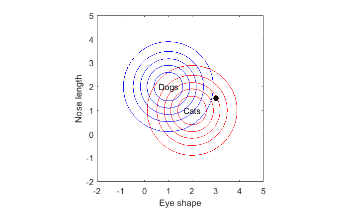
We can compare the likelihoods that each class would generate such an animal:

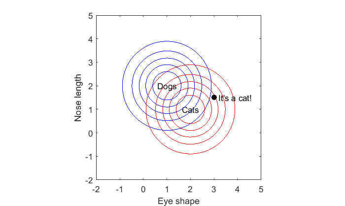
px1 = mvnpdf(x,m1);
px2 = mvnpdf(x,m2);

disp(sprintf('Likelihood Cat: %3.3f',px1));
disp(sprintf('Likelihood Dog: %3.3f',px2));

if px1 > px2
    text(x(1),x(2),'  It''s a cat!');
else
    text(x(1),x(2),'  It''s a dog!');
end

Likelihood Cat: 0.085
Likelihood Dog: 0.019

Decision boundary

Somewhere between the world of dogs and cats there is ambiguity. This is the region where the likelihoods for the two classes are equal. We can see this by finding where our probability matrices p1 and p2 are equal to zero.

More specifically, we can find where the log of their ratios are 0. This can be visualized with a contour plot with contour lines set near zero:

contour(xx(1,:),yy(:,1),log(p1./p2),linspace(-.01,.01,5),'Color','k');

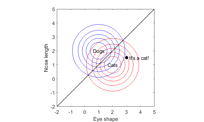
This is the decision boundary. Anything below it is most likely a cat, and anything above it is most likely a dog. It should make sense for this example why the decision boundary is a straight line passing right between the means of the two classes.

The decision boundary is always a straight line when the covariance matrices for the two classes are the same:

m1 = [2,1];
C1 = [1,-.75;
    -.75,1];

m2 = [1,2];
C2 = C1;  % Covariances are the same


p1 = mvnpdf(X,m1,C1);
p1 = reshape(p1,size(xx));

p2 = mvnpdf(X,m2,C2);
p2 = reshape(p2,size(xx));

figure(1)
clf
contour(xx(1,:),yy(:,1),p1,cLevels,'Color','r');

text(m1(1),m1(2),'Cats','HorizontalAlignment','center');
hold on

contour(xx(1,:),yy(:,1),p2,cLevels,'Color','b');
text(m2(1),m2(2),'Dogs','HorizontalAlignment','center');
contour(xx(1,:),yy(:,1),log(p1./p2),linspace(-.01,.01,5),'Color','k');

xlabel('Eye shape')
ylabel('Nose length');

axis equal

Play with the means, m1 and m2, and the covariance matrix, S1, to verify that the decision boundary is always a straight line.

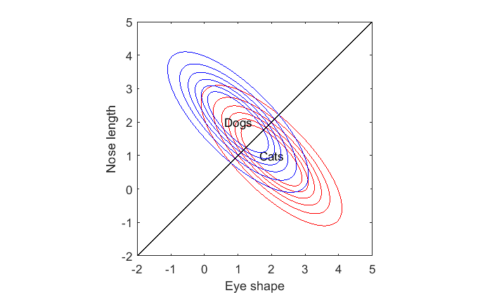
Unequal covariance matrices

Things get interesting when we allow for unequal covariance matrices. Suppose again that for cats there is a negative correlation between eye-shape and nose length. But also let's say that there is a positive correlation for dogs, so that dogs that have long noses also tend to have more oval-shaped eyes. Here's what this might look like:

m1 = [2,1];
C1 = [1,-.75;
    -.75,1];

m2 = [1,2];
C2 = [1,.75,
    .75,1];

p1 = mvnpdf(X,m1,C1);
p1 = reshape(p1,size(xx));

p2 = mvnpdf(X,m2,C2);
p2 = reshape(p2,size(xx));

figure(1)
clf
contour(xx(1,:),yy(:,1),p1,cLevels,'Color','r');

text(m1(1),m1(2),'Cats','HorizontalAlignment','center');
hold on

contour(xx(1,:),yy(:,1),p2,cLevels,'Color','b');
text(m2(1),m2(2),'Dogs','HorizontalAlignment','center');
contour(xx(1,:),yy(:,1),log(p1./p2),linspace(-.01,.01,5),'Color','k');

xlabel('Eye shape')
ylabel('Nose length');

axis equal

Check out the decision boundary. It's curved. In fact it's a hyperbola. Fun fact: the decision boundary for any pair of bivariate distribution will be a quadratic of the form ax^2 + bx^2 + cxy + d = 0. If you remember your geometry, the solution to this equation will be a conic section which means that the boundary will either be a line, circle, ellipse, parabola or hyperbola.

Hypberbolas have two curves. The curve that passes between the means for dogs and cats makes sense. But what about the other one? It says that if you have an animal with a very round eye-shape and a very short nose, then it must be a cat! It's interesting because the average dog has rounder eyes and shorter noses than cats. But an extremely dog-like animal will be classified as a cat.

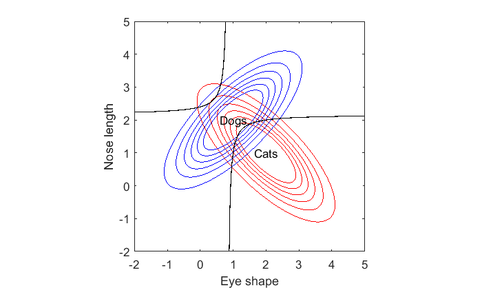
Play around with some means and covariances to see if you can get any interesting decision boundaries. You can get a circle or ellipse if the means are the same but the covariances are different in scale:

m1 = [1,1];
C1 = [1,0;
    0,1];

m2 = [1,1];
C2 = [.5,0,
    0,.5];

Does this decision boundary make sense? Can you think of any real-world examples where this might be the case?

Three classes in two dimensions

Finding class boundaries naturally extends to more than two classes. Let's consider a third animal, weasels, that have oval eyes and long noses (they look to me both cat and dog-like). Let's assume the eye-shape of weasels have a mean of 1.5 and the nose length has a mean of 1.5, and that these features don't correlate but have a small amount of variance. We'll assume the previously correlated features for cats and dogs:

% cats
m1 = [2,1];
C1 = [1,-.75;
    -.75,1];

% dogs
m2 = [1,2];
C2 = [1,.75,
    .75,1];

% *new* weasels!
m3 = [2,2];
C3 = [.25,0,
    0,.25];

p1 = mvnpdf(X,m1,C1);
p1 = reshape(p1,size(xx));

p2 = mvnpdf(X,m2,C2);
p2 = reshape(p2,size(xx));

p3 = mvnpdf(X,m3,C3);
p3 = reshape(p3,size(xx));

figure(1)
clf
hold on

contour(xx(1,:),yy(:,1),p1,cLevels,'Color','r');
contour(xx(1,:),yy(:,1),p2,cLevels,'Color','b');
contour(xx(1,:),yy(:,1),p3,cLevels,'Color','g');

text(m1(1),m1(2),'Cats','HorizontalAlignment','center');
text(m2(1),m2(2),'Dogs','HorizontalAlignment','center');
text(m3(1),m3(2),'Weasels','HorizontalAlignment','center');

xlabel('Eye shape')
ylabel('Nose length');

axis equal

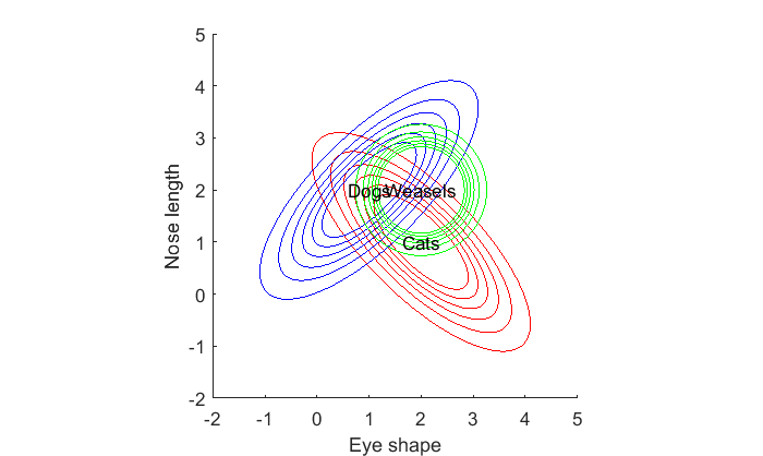
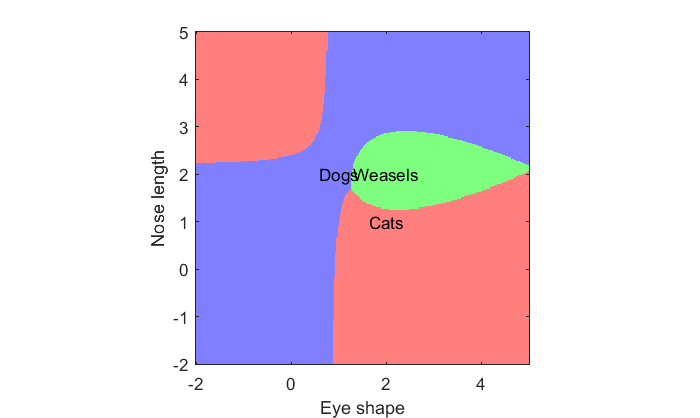
How should we classify any given animal in this three-class feature space? The logic is the same. For any given animal, we find the likelihood that each class generated that animal and assign the class to the most likely one.

Using a contour plot to show the decision boundary for more than three classes gets complicated. Instead, we can simply make an image and color it according to the class that has the maximal likelihood:

% Make a 3-row vector, where each row corresonds to a pixel in the image,
% then take the maximum for each column (pixel)
[tmp,classNum] = max([p1(:)';p2(:)';p3(:)']);

% Reshape the vector back into an image:
classNum = reshape(classNum,size(p1));

% Show the image with a colormap
figure(2)
clf
image(xx(1,:),yy(:,1),classNum)
colormap([1,.5,.5;.5,.5,1;.5,1,.5]);
hold on

% label things.
text(m1(1),m1(2),'Cats','HorizontalAlignment','center');
text(m2(1),m2(2),'Dogs','HorizontalAlignment','center');
text(m3(1),m3(2),'Weasels','HorizontalAlignment','center');
set(gca,'YDir','normal');
xlabel('Eye shape');
ylabel('Nose length');
axis tight
axis equal

To do:

1. Play around with different means and covariance matrices for the three classes and look at the category boundaries.

2. Add a fourth category (badgers?) and see how the category boundaries are affected.

3. Think about what the boundaries would look like with three feature dimensions instead of two.

Discriminant Analysis Classification

Now that we have a feel for what these boundaries look like for known population distributions, we'll now turn to what to do when we only have samples from such populations.

Like most inferential statistics, discriminant analysis classification uses the statistics from our samples as our best guess of the population parameters. We'll then define the boundaries like we did above, but based on our sample statistics.

Discriminant analysis classification is a 'parametric' method, meaning that the method relies on assumptions made about the population distribution of values along each dimension. Specifically, the method assumes that values are distributed normally.

For the first example, let's assume the two classes of dogs and cats, and assume that eye shape and nose length are both distributed normally with standard deviations of 1. We'll also assume that there is no correlation between nose length and eye shape within each animal class. Do you remember what the decision boundary should look like?

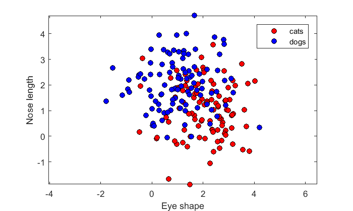
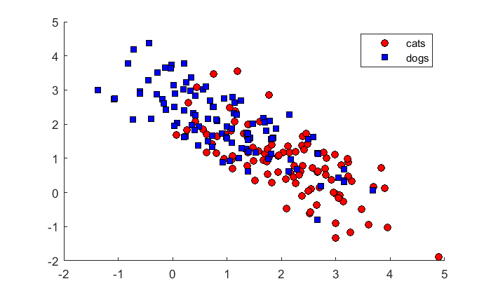
Let's generate a sample of values for 100 cats and 100 dogs.

n = 100;  % number of animals per class

m1 = [2,1];  %  means for cats: eye shape = 2, nose length = 1
C1 = [1,0;
    0,1];  % covariance for cats

m2 = [1,2];  %  means for dogs: eye shape = 1, nose length = 2
C2 = [1,0
    0,1];  % covariance for dogs
x1 = mvnrnd(m1,C1,n);
x2 = mvnrnd(m2,C2,n);

'x1' holds the values for cats, where the first column is for eye shape and the second is nose length. x2 is the same, but for dogs.

Here's a scatterplot showing the samples along the two dimensions:

figure(1)
clf
h(1)= plot(x1(:,1),x1(:,2),'ko','MarkerFaceColor','r');
hold on
h(2) = plot(x2(:,1),x2(:,2),'ko','MarkerFaceColor','b');
axis equal
xlabel('Eye shape');
ylabel('Nose length');
legend('cats','dogs','Location','NorthEast');

MATLAB's 'fitcdiscr' function

Discriminant analysis will calculate the means and covariances for the samples, and use them to define boundaries much like we did above for the population parameters. This is done with the 'fitcdiscr' function which is part of the statistics toolbox.

'fitcdiscr' stands for 'Fit discriminant analysis classifier'. To classify cats and dogs, we have to adapt our data into a specific format. First, we need a single matrix, X, for which each row is a different animal (sample), and each column is a dimension (eye-shape and nose-length). The matrix holds the values for all classes:

X = [x1;x2];

The second thing that 'fitcdiscr' needs is a list of classes that each animal belongs to. For our example, the first 100 animals are cats, and the next 100 are dogs:

c = [ones(n,1);2*ones(n,1)];

'fitcdiscr' uses object oriented programming. To use it we first call the function to obtain and object to be used later. You can think of this function as 'training' the classifier based on our data. We can use any name for the resulting object, so we'll use the name 'lda' here:

lda = fitcdiscr(X,c);

Here's the name of the class of this object, if you're interested:

class(lda)

ans =

ClassificationDiscriminant

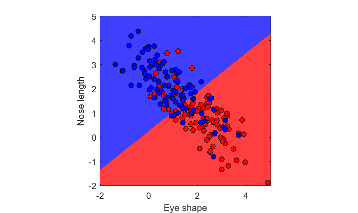
We can do a bunch of stuff with this object. First, let's try to classify our existing set of animals using the 'predict' function:

pred_c = predict(lda,X);

The output is a list of 1's and 2's which are the best guesses for each sample. Let's plot these best guesses on a scatterplot:

figure(2)
clf
hold on
h(1) = plot(X(pred_c==1,1),X(pred_c==1,2),'ko','MarkerFaceColor','r');  % cats
h(2) = plot(X(pred_c==2,1),X(pred_c==2,2),'ks','MarkerFaceColor','b');  % dogs
axis equal
xlabel('Eye shape');
ylabel('Nose length');
legend('cats','dogs','Location','NorthEast');

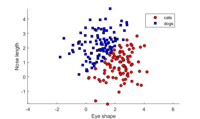
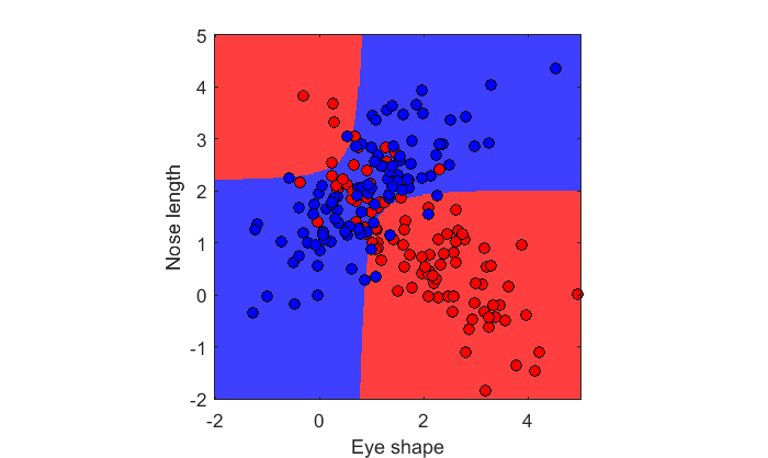
By default 'fitcdscr' uses a 'linear classifier' which assumes, like our current example, that our samples are drawn from bivariate Gaussians with equal covariances. As we discussed above this always generates a straight line as a classification boundary, which you can clearly see.

Note that due to the overlap in the distributions that with a linear classifier, some dogs will be classified as cats and vice versa. This is the nature of classification. It's not always 100% accurate if the distributions overlap.

Let's calculate the accuracy by comparing 'pred_c' to 'c':

accuracy = mean(pred_c==c)

accuracy =

    0.7800

The linear classifier got it right about 75% of the time. We can also use the 'resubLoss' function which gives you the proportion of wrong classifications, which is about 25%

resubLoss(lda)

ans =

    0.2200

These should add up to 1:

accuracy + resubLoss(lda)

ans =

    1.0000

We can classify novel animals too with the 'predict' function:

newX = [2,1];  % An animal with oval eyes and a short nose
pred_c = predict(lda,newX)

if pred_c == 1
    disp('It''s a cat!');
else
    disp('It''s a dog!');
end

pred_c =

     1

It's a cat!

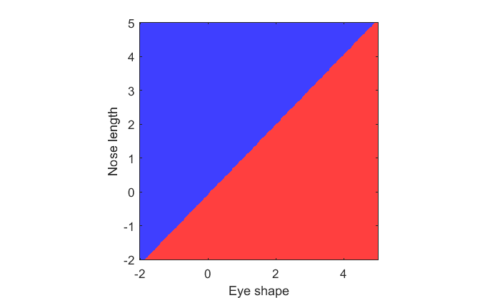
To visualize the decision rule, we can classify animals for every pixel in our [xx,yy] grid and show it as an image:

pred_grid = predict(lda,[xx(:),yy(:)]);
pred_grid = reshape(pred_grid,size(xx));

figure(3)
clf
image(xx(1,:),yy(:,1),pred_grid)
colormap([1,.25,.25;.25,.25,1]);

axis equal
axis tight
set(gca,'YDir','normal');
xlabel('Eye shape');
ylabel('Nose length');

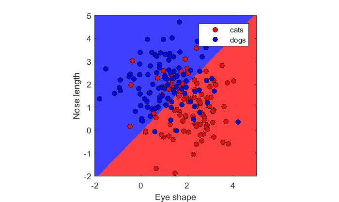
We can plot the original samples on top to see which animals are misclassified:

hold on
h(1)= plot(x1(:,1),x1(:,2),'ko','MarkerFaceColor','r');
h(2) = plot(x2(:,1),x2(:,2),'ko','MarkerFaceColor','b');

legend('cats','dogs','Location','NorthEast');

Unequal population variances:

for example, it could be that eye-shape is much less variable than nose-length for both cats and dogs. Let's see how this affects the decision boundary. We'll do this by adjusting the 's1' and 's2' vectors that define the population standard deviations.

n = 100;  % number of animals per class
m1 = [2,1];
C1 = [1,-.75;
    -.75,1];

m2 = [1,2];
C2 = C1;  % Covariances are the same

x1 = mvnrnd(m1,C1,n);
x2 = mvnrnd(m2,C2,n);

figure(1)
clf
hold on
h(1)= plot(x1(:,1),x1(:,2),'ko','MarkerFaceColor','r');
h(2) = plot(x2(:,1),x2(:,2),'ks','MarkerFaceColor','b');

legend('cats','dogs','Location','NorthEast');

We'll find the decision boundary again. I've written a function 'showDecisionBoundary' that generates the image, because we'll be doing it a few more times:

c = [ones(n,1);2*ones(n,1)];
X = [x1;x2];
lda = fitcdiscr(X,c);
figure(2)
clf
showDecisionBoundary(lda,X,c)

The decision boundary is still a straight line. Notice the slope though. The population parameters predict decision boundary along y=x. This boundary is slightly different - that's because it's based on the sample statistics and not the population parameters. The sample statistics are:

mean(x1)
cov(x1)

mean(x2)
cov(x2)

ans =

    2.0752    0.8918


ans =

    0.9225   -0.6906
   -0.6906    0.9771


ans =

    0.9179    2.0390


ans =

    1.1324   -0.7925
   -0.7925    0.9387

Unequal and correlated population variances: Quadratic discriminant analysis

We'll now sample data from populations where cats with more oval-shaped eyes have shorter noses, and dogs with more oval-shaped eyes have longer noses:

% cats
m1 = [2,1];
C1 = [1,-.75;
    -.75,1];

% dogs
m2 = [1,2];
C2 = [1,.75,
    .75,1];
x1 = mvnrnd(m1,C1,n);
x2 = mvnrnd(m2,C2,n);

figure(1)
clf
hold on
h(1)= plot(x1(:,1),x1(:,2),'ko','MarkerFaceColor','r');
h(2) = plot(x2(:,1),x2(:,2),'ks','MarkerFaceColor','b');

legend('cats','dogs','Location','NorthEast');

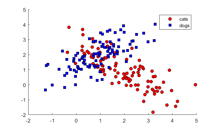
Here's the linear discriminant classification result:

c = [ones(n,1);2*ones(n,1)];
X = [x1;x2];
lda = fitcdiscr(X,c);
figure(2)
clf
showDecisionBoundary(lda,X,c)

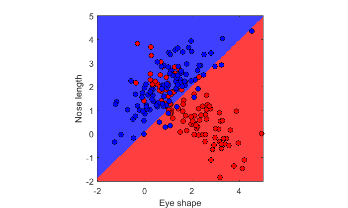
Does this look right? What should the decision boundary look like for the population parameters?

The 'fitcdiscr' function allows for unequal covariances by changing the 'DiscrimType' from the default of 'linear' to 'quadratic':

c = [ones(n,1);2*ones(n,1)];
X = [x1;x2];
lda = fitcdiscr(X,c,'DiscrimType','quadratic');
figure(2)
clf
showDecisionBoundary(lda,X,c)

This looks a lot more like the hyperbolic decision boundary we calculated earlier from the population.

Weasels!

fitcdiscr naturally generalizes to more than two classes. Here is some data generated from the third class, weasels:

% *new* weasels!
m3 = [2,2];
C3 = [.25,0,
    0,.25];

x3 = mvnrnd(m3,C3,n);

% New X matrix and c vector
c = [ones(n,1);2*ones(n,1);3*ones(n,1)];
X = [x1;x2;x3];

lda = fitcdiscr(X,c,'DiscrimType','quadratic');
figure(2)
clf
showDecisionBoundary(lda,X,c,{'cats','dogs','weasels'})

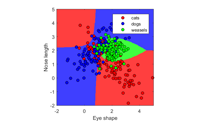
Here's the accuracy of classifying the known animals

disp(sprintf('Accuracy: %5.2f%%',100*(1-resubLoss(lda))));

Accuracy: 74.67%

Cross-validation

The accuracy calculated above really isn't a good measure of how good the classification is for a real data set. That's because using data to classify itself is circular. Consider the null hypothesis where all three classes have the same population parameters:

m1 = [0,0];
C1 = [1,0,
    0,1];

m2 = m1;
C2 = C1;

m3 = m1;
C3=  C1;

x1 = mvnrnd(m1,C1,n);
x2 = mvnrnd(m2,C2,n);
x3 = mvnrnd(m3,C3,n);

c = [ones(n,1);2*ones(n,1);3*ones(n,1)];
X = [x1;x2;x3];
lda = fitcdiscr(X,c,'DiscrimType','quadratic');
disp(sprintf('Accuracy: %5.2f%%',100*(1-resubLoss(lda))));

Accuracy: 38.33%

Chance accuracy for three classes should be 33%, but if you re-run the above cell you'll find accuracy is always above that. That's because the algorithm is using the same data to define the boundaries as it is to classify.

An unbiased way would be to use data from one experiment to define the boundaries - sometimes called a training set, and another independent data set, called the test set, to test the accuracy based on this training set.

Here's a new fake data set under the null hypothesis:

x1new = mvnrnd(m1,C1,n);
x2new = mvnrnd(m2,C2,n);
x3new = mvnrnd(m3,C3,n);
Xnew = [x1new;x2new;x3new];
pred_c = predict(lda,Xnew);
disp(sprintf('Accuracy: %5.2f%%',100*mean(pred_c==c)));

Accuracy: 29.33%

Run it again and again and you'll see that classifying a new data set based on the previous training set will give you an average of 33% accuracy.

But running a new experiment is expensive. An alternative is to split the data into two parts and then treat one part as training and the other as the test set. This can be done multiple times for a single data set by dividing the data differently each time.

There are various ways to do this. The most popular is the 'k-fold' cross validation procedure. It randomly divides the data set into k non-overlapping subsets. Each subset has roughly equal size and roughly the same class proportions as in the training set. The algorithm then removes one subset at a time, trains the classification model using the other k-1 subsets, and uses the trained model to classify the removed subset.

Matlab's 'cvpartition' generates an object that holds a random partitioning of your data into a training set and test set:

cp = cvpartition(c,'KFold',10);

'crossval' takes this object and and returns yet another object:

cvlda = crossval(lda,'CVPartition',cp);

Finally, 'kfoldLoss' takes the object from 'crossval' and pulls the proportion of errors out of the object. Accuracy is 1 minus this value:

ldaCVErr = kfoldLoss(cvlda);
disp(sprintf('Cross-validation accuracy: %5.2f%%',100*(1-ldaCVErr)));

Cross-validation accuracy: 27.67%

In addition to 'KFold', other cross validation partition methods are 'HoldOut' and 'LeaveOut'. They're all closely related. More can be found with:

doc cvpartition

More than two feature dimensions: Multi-Voxel Pattern Classification

Now we know how to classify cats, dogs and weasels. Let's move on to an application that's more relevant to work going on in our lab - something called 'Multi-Voxel Pattern Classification', or MVPA.

The short history of MVPA is that in the early days of fMRI it was assumed that the signal didn't contain information about stimulus properties that are encoded at a spatial resolution smaller than the size of a voxel. For example, it is known in primates that neurons in area V1 are selective to the orientation of a stimulus. Similarly tuned neurons cluster together, forming 'pinwheeels' of selectivity so that orientation preferences varies continuously as you traverse a little circle on the surface of the cortex.

The sizes of these pinwheels are on the order of 1mm in the macaque, and fMRI voxels are around 3mm cubed. It was therefore assumed that the response from a single fMRI voxel wouldn't depend much on the orientation of the stimulus presented because the selectivity of the population of neurons underlying its response would be roughly equal across orientations.

That all changed in 2005 when Yukiyasu Kamitani and Frank Tong showed that there was indeed information about orientation encoded across the pattern of responses in V1 voxels. And you may have guessed, they showed this by demonstrating that a pattern classification algorithm could be used to predict the orientation a test stimulus based on responses to a training set.

This opened the door for studying the response and perception of a whole new set of stimulus properties that were previously believed to organized at too small of a spatial scale. MVPA has since been used to study motion, color, object perception and even personality.

Here we'll have some fun and generate voxel responses to stimuli of various orientations using a model of the pinwheel map on the cortical surface.

Here's a fake pinwheel map showing the orientation preference on the surface of the cortex. Colors represent different preferred orientations. Units are in millimeters.

The algorithm that generates the map isn't directly relevant to this tutorial so I've buried it in the function 'makePinwheelMap'. If you're interested, it's based on an article by Rojer and Schwartz (Biol Cybern, 1990).

nVox = [1,2];
voxSize = 3;
nAngles =2;

[nn,img,xax,yax] = makePinwheelMap(nVox,voxSize,nAngles);

figure(1)
clf
image(xax,yax,img);
colormap(hsv(64));
axis equal
axis tight
set(gca,'XTick',0:voxSize:voxSize*nVox(2));
set(gca,'YTick',0:voxSize:voxSize*nVox(1));
grid

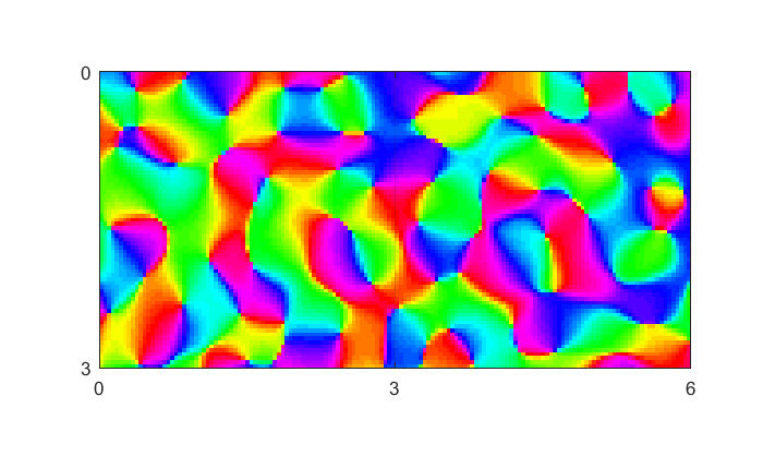
The gridlines are 3mm apart, so they represent separate fMRI voxels. You can see that there are two voxels represented here.

The function also returns a prediction of each voxel's response to different orientations. It's stored in the 2D matrix 'nn' where the columns represent different voxel responses and the rows are different stimulus orientations.

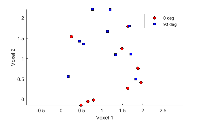
Let simulate an experiment where we're trying to predict the orientation of a stimulus based on the response to two fMRI voxels. In our 'experiment', subjects will be presented stimuli having one of two orientations (0 or 90 degrees) in a given scan. Five scans will be repeated for each orientation.

We'll use the output of the model, in the nn matrix, as our population mean responses from the two voxels to the two orientations. We'll add Gaussian noise to generate the responses to the five repeated runs.

The model predicts a mean response of 1 across orientations for each voxel. Our Gaussian noise will have a standard deviation of 0.5 as well, which is a fairly accurate measure of run-to-run variability in fMRI data.

n=10;  %Number of experimental runs

m1 = nn(:,1)';
C1 = .5*[1,0,
    0,1];

m2 = nn(:,2)';
C2 = C1;

m3 = m1;
C3=  C1;

x1 = mvnrnd(m1,C1,n);
x2 = mvnrnd(m2,C2,n);

c = [ones(n,1);2*ones(n,1)];
X = [x1;x2];

Because we have two voxels and two orientations, we can plot our voxel responses as a scatterplot as before:

figure(2)
clf
hold on
h(1)= plot(x1(:,1),x1(:,2),'ko','MarkerFaceColor','r');
h(2) = plot(x2(:,1),x2(:,2),'ks','MarkerFaceColor','b');

legend('0 deg','90 deg','Location','NorthEast');
xlabel('Voxel 1');
ylabel('Voxel 2');
axis equal

We'll use the K-fold cross validation to determine our classification accuracy.

lda = fitcdiscr(X,c,'DiscrimType','linear');
cp = cvpartition(c,'KFold',10);
cvlda = crossval(lda,'CVPartition',cp);
ldaCVErr = kfoldLoss(cvlda);
disp(sprintf('Cross-validation accuracy: %d, %5.2f%%',i,100*(1-ldaCVErr)));

Cross-validation accuracy: 1, 65.00%

With only two voxels and 10 runs you can see that classification accuracy is going to be pretty poor.

But usually there are hundreds of voxels in a given region of interest. Kamitani and Tong had about 400 voxels in V1, and tried to classify using eight different stimulus orientations. You'll see that accuracy improves dramatically:

voxSize = 3;
nVox = [20,20];
nAngles = 8;

[nn,img,xax,yax] = makePinwheelMap(nVox,voxSize,nAngles);
figure(1)
clf
image(xax,yax,img);
colormap(hsv(64));
axis equal
axis tight
set(gca,'XTick',0:voxSize:voxSize*nVox(2));
set(gca,'YTick',0:voxSize:voxSize*nVox(1));
grid

n=10;  % Number of experimental runs
C = eye(prod(nVox));
X = [];
c = [];
for i=1:nAngles
    m = nn(i,:); % Population mean for this angle, across voxels
    X = [X; mvnrnd(m,C,n)];
    c = [c;i*ones(n,1)];
end

Again,we'll use the K-fold cross validation to determine our classification accuracy.

lda = fitcdiscr(X,c,'DiscrimType','linear');
cp = cvpartition(c,'KFold',10);
cvlda = crossval(lda,'CVPartition',cp);
ldaCVErr = kfoldLoss(cvlda);
disp(sprintf('Cross-validation accuracy: %5.2f%%',100*(1-ldaCVErr)));

Cross-validation accuracy: 72.50%

for i = 1:cp.NumTestSets
    trIdx = cp.training(i);
    teIdx = cp.test(i);
    ytest = classify(X(teIdx,:),X(trIdx,:),...
		 c(trIdx,:),'linear');
    err(i) = sum(~strcmp(ytest,c(teIdx)));
end
cvErr = sum(err)/sum(cp.TestSize);

Error using classify (line 228)
The pooled covariance matrix of TRAINING must be positive definite.

Error in Lesson_20 (line 1002)
    ytest = classify(X(teIdx,:),X(trIdx,:),...

Problems

1) How does cross-validation classification accuracy increase with the number of voxels? Does the accuracy saturate?

2) Test the cross-validation classification accuracy under the null hypothesis that there is no pattern information about orientation across voxels. I can think of two ways:

a) Replace X with randn(size(X)) and repeatedly run the cross-validation analysis. Calculate the mean accuracy. It should be 12.5 percent (100*1/8)

b) Shuffle the class identifier variable with c = c(randperm(length(c)))

Published with MATLAB® R2015b