Lesson 5: Fitting the psychometric function

In this lesson we'll calculate the coherence threshold from sample psychometric function data. This involves fitting the trial-by-trial results with a parametric function (the Weibul function) using a 'maximum likelihood' procedure and picking off the coherence level that predicts 80% correct performance.

Contents

The Weibull function

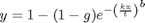
A standard function to predict a psychometric function from a 2AFC experimenet like the one we've been doing is called the 'Weibull' cumulative distribution function. It has the general form:

where x is the stimulus intensity and y is the percent correct. Lambda and k are free parameters. A reparameterized version for our purposes is:

where

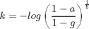
With this parameterization, g is the performance expected at chance (0.5 in our case of 2AFC), t is the threshold, and a is the performance level that defines the threshold. That is, if x=t then y=a. The parameter b determines the slope of the function.

I've provided this function for you. It's called Weibull.m

help Weibull

 y = Weibull(p,x)
 
 Parameters:  p.b slope
              p.t threshold yeilding ~80% correct
              x   intensity values.

Let's plot a family of curves for a fixed threshold (p.b) and varying slope (p.t). We'll plot the curves on a log-x axis.

x = linspace(.05,1,101);
p.t = .5;
bList = 1:4;
figure(1)
clf
subplot(1,2,1)
y = zeros(length(bList),length(x));
for i=1:length(bList)
    p.b = bList(i);
    y(i,:) = Weibull(p,x);
end
plot(log(x),y')
logx2raw;
legend(num2str(bList'),'Location','NorthWest');
xlabel('Intensity');
ylabel('Proportion Correct');
title('Varying b with t=0.3');
%
% Note how that the slopes vary, but all curves pass through the same
% point.  This is where x=p.t and y =a.  In our case, x=0.3 and y ~= .8.
%
% Next we'll plot a family of curves for a fixed slope(p.t) and varying
% threshold (p.t).

p.b = 2;
tList = [.1,.2,.4,.8];
subplot(1,2,2)
y = zeros(length(tList),length(x));
for i=1:length(tList)
    p.t = tList(i);
    y(i,:) = Weibull(p,x);
end
plot(log(x),y')

legend(num2str(tList'),'Location','NorthWest');
xlabel('Intensity');
ylabel('Proportion Correct');
set(gca,'XTick',log(tList));
logx2raw
title('Varying t with b=2');

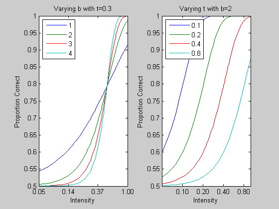
See how for each curve,when the intensity is equal to the threshold (p.t), then the percent correct is ~80%. So the variable p.t determines where on the x-axis the curve reaches 80%.

By varying the two parameters, p.b and p.t, we can generate a whole family of curves that are good at describing psychometric functions in a 2AFC experiment.

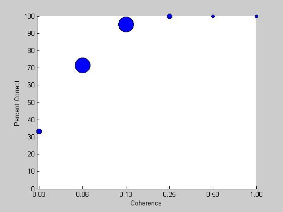
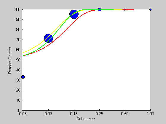
Let's draw an example Weibull function on top of some psychometric function data generated in the previous lesson. I've written a function called 'plotPsycho' that is based on the psychometric plotting code in Lesson 4.

% Load in your results from Lesson 4.
load resultsStaircase

% Strip out the trials where there was an invalid response (if there are any).
goodTrials = ~isnan(results.response);
results.response = results.response(goodTrials);
results.intensity = results.intensity(goodTrials);

figure(1)
plotPsycho(results,'Coherence')

A first guess at a set of parameters

Then we'll chose some parameters for a slope and threshold. It looks like the threshold should be around 0.1. We'll pick a slope of 2.

pGuess.t =0.1;
pGuess.b = 2;

x = exp(linspace(log(min(results.intensity)),log(max(results.intensity)),101));

%x = logspace(log(min(results.intensity)),log(max(results.intensity)),101);
y= Weibull(pGuess,x);

hold on

plot(log(x),y*100,'r-','LineWidth',2);

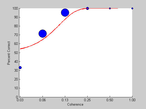
This looks like a pretty good fit. But is this the best we can do? To answer this question we need a measure of how well the curve fits the data. A common measure for curve fitting is a sums-of-squared error (SSE), which is the sum of the squared deviations between the curves and the data points. However, for percent-correct data like this, SSE is not appropriate because deviations along the percent-correct do not have equal weights. A 10% deviation for performance around 50% is less meaningful than a 10% deviation around 90%.

Likelhihood

For percent-correct data (or any data generated through a binary process), the appropriate measure is 'likelihood'. Here's how it's calculated;

For a given trial, i, at a given stimulus intensity, xi, the Weibull function predicts the probability that the subject will get the answer correct. So if the subject did get respond correctly, then the probability of that happening is:

Where xi is the intensity of the stimulus at trial i, and W(xi) is the Weibull function evalulated at that stimulus intensity. The probability of an incorrect answer is simply:

Assuming that all trials in the staircase are independent, then for a given Weibull function, the probability of observing the entire sequence of subject responses is:

for correct trials, and

for incorrect trials.

If we let ri = 1 for correct trials and ri=0 for incorrect trials, like the vector results.response, then a simple way to calculate the probability of observing the whole sequence in one line is:

Here's how to do it in Matlab with our data set:

Evaluate the Weibull function for the stimulus intensities used in the staircase

y = Weibull(pGuess,results.intensity);

%Calculate the likelihood of observing our data set given this particular
% choice of parameters for the Weibull:

likelihood = prod( y.^results.response .* (1-y).^(1-results.response))

likelihood =

  3.0916e-010

We want to choose values of p.t and p.b to make this number as large as possible. This is a really small number - sort of surprising since we thought that our choice of parameters for the Weibull was reasonably good. The reason for this small number is that the product of a bunch of numbers less than 1 gets really small. To avoid this, we can take the logarithm of the equation above - this expands the range of small numbers so that we're not going to run into machine tolerance problems:

The Matlab calculation of this is:

logLikelihood = sum(results.response.*log(y) + (1-results.response).*log(1-y))

logLikelihood =

   NaN

NaN? Turns out that this calculation can fail if the values of y reach 1 because the log of 1-y can't be computed. The way around this is to pull the values of y away from zero and 1 like this:

y = y*.99+.005;

This is called a 'correction for guessing' and it deals with the fact that subjects will never truly perform at 100% for any stimulus intensity because human subjects will always make non-perceptual errors, like motor errors, or have lapses in attention.

Here's a re-calculation of the log likelihood:

logLikelihood = sum(results.response.*log(y) + (1-results.response).*log(1-y))

logLikelihood =

  -22.0208

This is a more reasonable magnitude to deal with. (It's negative because the log of a number less than 1 is negative). Let's calulate the log likelihood for a different set of Weibull parameters:

I've written a function called 'fitPsychometricFunction.m' that makes this calculation. It takes in as arguments the structure 'p' holding the function's parameters, the results structure, and a string containing the name of the function to use ('Weibull') in our case. It's almost exactly the same as the calculation above except that it reverses the sign (multiplies the log likelihood by -1) of the log likelihood. This provides a positive number where smaller numbers mean better fits. This is compatible with the optimization search algorithms that we'll discuss in a bit.

Here's how to use it.

fitPsychometricFunction(pGuess,results,'Weibull')

ans =

   22.0208

Note that the value is exactly the negative of the previous calculation.

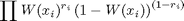
Let's try for a better fit:

pBetter.t =0.075;
pBetter.b = 2;
fitPsychometricFunction(pBetter,results,'Weibull')

ans =

   21.1564

It's a smaller number which means it's an even better fit. We can visualize this by plotting this new prediction in yellow on the old graph:

y = Weibull(pBetter,x);
hold on
plot(log(x),100*y,'y-','LineWidth',2);

The log-likelihood surface

How do we find the parameters that maximize the log likelihood? Matlab has a function that does this in a sophisticated way. But for fun, let's just look at what the log likelood is for a range of values. Since there are two parameters, we can think of the log likelihood as being a 'surface' with p.b and p.t being the x and y axes.

List of b and t values:

bList = linspace(0,4,31);
tList = exp(linspace(log(.05),log(0.25),31));

% Loop through the lists in a nested loop to evaluate the log likelihood
% for all possible pairs of values of b and t.

logLikelihoodSurface = zeros(length(bList),length(tList));

for i=1:length(bList)
    for j=1:length(tList)
        p.b = bList(i);
        p.t = tList(j);
        y = Weibull(p,results.intensity);
        logLikelihoodSurface(i,j) = fitPsychometricFunction(p,results,'Weibull');
    end
end

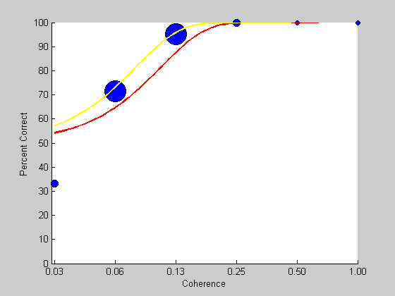
We can visualize the surface by using a contour plot

figure(2)
clf
contour(log(tList),bList,logLikelihoodSurface,linspace(20,30,50))
xlabel('t');
ylabel('b');
logx2raw

We can plot the most recent set of parameters as a symbol on this contour plot.

hold on
plot(log(pGuess.t),pGuess.b,'o','MarkerFaceColor','r');
plot(log(pBetter.t),pBetter.b,'o','MarkerFaceColor','y');

This figure is like a topographical map. Each line represents the values of b and t that produce an equal value for log likelehood. The fourth argument into 'contour' is a list of these values.

The figure shows a series of concentric shapes with the smallest circling around t=0.12 and b = 1.6. This is the 'bottom' of our surface and is close to the best choice of Weibull parameters.

Matlab's 'fminsearch' routine and 'fit.m'

Searching through the entire grid of possible parameters is clearly an inefficient strategy (especially if there are even more parameters to deal with). Fortunately there is a whole science behind finding the best parameters to minimize a function, and Matlab has incorporated some of the best in their function called 'fminsearch'.

I find the way fminsearch is called a bit inconvenient. It allows me to put all variables for the function into a structure (feeding my obsession with structures), and it makes it easy to keep some parameters fixed and others to vary. So I've written a function that calls fminsearch called 'fit.m'. Here's how to use it:

help fit

 [params,err] = fit(funName,params,freeList,var1,var2,var3,...)
 
 Helpful interface to matlab's 'fminsearch' function.
 
 INPUTS
  'funName':  function to be optimized.  Must have form err = <funName>(params,var1,var2,...)
  params   :  structure of parameter values for fitted function
      params.options :  options for fminsearch program (see OPTIMSET)
  freeList :  Cell array containing list of parameter names (strings) to be free in fi
  var<n>   :  extra variables to be sent into fitted function
 
 OUTPUTS
  params   :  structure for best fitting parameters 
  err      :  error value at minimum
 
 See 'FitDemo.m' for an example.
 
 Written by Geoffrey M. Boynton, Summer of '00

    Overloaded methods:
       gmdistribution/fit

The first argument into 'fit' is the name of the function to be minimized. In our case it's 'FitPsychometricFunction'. This function must have the specific form of the output being the value to be minimized and the first input argument being a structure containing the parameters that can vary. The other input arguments can have any form.

The next argument input into 'fit' is the starting set of parameters in a structure. The third argument is a cell array containing a list of fields in this structure that you want to let vary.

The remaining inputs are the same inputs that you'd put into the function to be minimized.

Here's how to use it for the Weibull function:

% Starting parameters
pInit.t = .1;
pInit.b = 2;

[pBest,logLikelihoodBest] = fit('fitPsychometricFunction',pInit,{'b','t'},results,'Weibull')

Fitting "fitPsychometricFunction" with 2 free parameters.

pBest = 

    t: 0.0809
    b: 2.4342


logLikelihoodBest =

   21.0326

Note that the parameters changed from the initial values, and the resulting log likelihood is lower than the two used earlier (using 'pGuess and pBetter'. Let's plot the best-fitting parameters on the contour plot in green:

plot(log(pBest.t),pBest.b,'o','MarkerFaceColor','g');

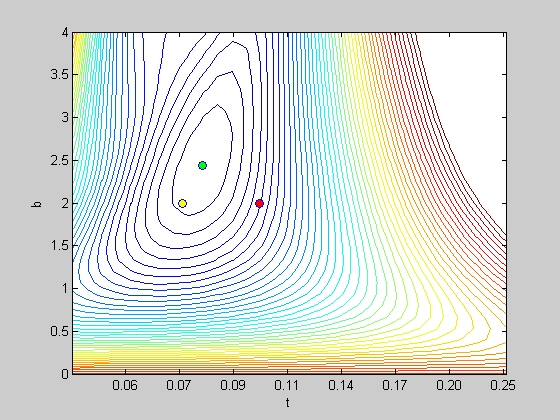
See how this best-fitting pair of parameters falls in the middle of the circular-shaped contour. This is the lowest point on the surface.

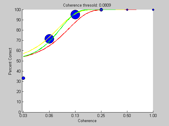
We now have the best fitting parameters. Let's draw the best predictions in green on top of the psychometric function data:

y = Weibull(pBest,x);
figure(1)
plot(log(x),100*y,'g-','LineWidth',2);

By design, the parameter 't' is the stimulus intensity that should predict 80% correct performance. We'll put the threshold in the title of the figure

title(sprintf('Coherence thresold: %5.4f',pBest.t));

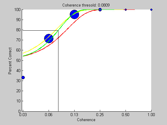
We can demonstrate this by drawing a horizontal line at ~80% correct to the curve and down to the threshold value on the x-axis:

plot(log([min(x),pBest.t,pBest.t]),100*(1/2)^(1/3)*[1,1,0],'k-');

Fixed and free parameters.

Suppose for some reason we want to find the threshold while fixing the slope to be 3. With 'fit' it's easy - all we do is change the list of 'free' parameters (the third argument sent to 'fit'):

% Initial parameters
pInit.t = .2;
pInit.b = 3;
[pBest,logLikelihoodBest] = fit('fitPsychometricFunction',pInit,{'t'},results,'Weibull')

Fitting "fitPsychometricFunction" with 1 free parameters.

pBest = 

    t: 0.0851
    b: 3


logLikelihoodBest =

   21.1573

We can show this on the contour plot. The threshold will be the best-fitting value along the horizontal line where b=1:

figure(2)
plot(log([min(tList),max(tList)]),pBest.b*[1,1],'k-')
plot(log(pBest.t),pBest.b,'ko','MarkerFaceColor','m');

Exercises

Published with MATLAB® 7.6