Chapter 10: Images and Movies
image – true color and colormaps
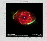
Let's begin by reading in and displaying an image.
close
all;
rgb
= imread('ngc6543a.jpg');
imread loads a image file. Sometimes you may need to also specify the file type that you want to read if it doesn't have an extension.
rgb=imread('ngc6543a',
'jpg');
Note that rgb is a 3D matrix, with the 3rd dimension representing the red green and blue
monitor values. Let's
now image this matrix.
figure(1);
image(rgb);
title('Cat''s eye Nebula');
Note how we use two "quotes" to produce a single quote on the title, this is to get around the issue that a single quote is used to mark the end of a string.
When we previously used the command image, we gave it a 2D matrix, where each value represented an entry into a colormap that specified the monitor RGB values. This time we are directly specifying the RGB values. This method of representing images is called true color.
If you want to read in an image that is stored using the colormap convention, it is done as follows:
[img, map]=imread('nofile.tiff');
In this case img
will be a 2D matrix, and map will be an m x 3 array containing the colormap.
Some file formats, like tiff can contain either colormap
or true color representation of data. You really need to just load it in, and
look to see whether the image is 2D or 3D.
One other thing you need to know about image is that it will represent images differently depending on whether the image matrix is stored as doubles or as uint8s (as you may recall, images are often saved as uint8 in order to save space). If you are having trouble using image when reading in a stored jpg or tiff image it's worth thinking about whether your image is actually in uint8 format.
The following table explains the options.
|
|
double |
uint8 |
|
colormap |
Image
matrix must be 2D and contain values in the range of 1:length(colormap) (usually 1:256). The
colormap must be an m
x 3
array with values that range between 0-1. |
Image
matrix must be 2D and contain values in the range of 0:255. The
colormap must be an m
x 3
array with values that range between 0-1. |
|
true color |
Image
matrix must be 3D (p x q x 3) with values that range
between 0-1 |
Image
matrix must be 3D (p x q x 3) with values that range
between 0-255. |
Saving images as tiff or jpeg
You can also write either colormap or true color images to a graphics file. Here, in NoiseImages.m we are going to create and save some random noise images. First we will create and save grayscale noise, using both colormap and true color techniques. Then we will create and save colored noise using just the true color technique (think about why we can't use the colormap technique to create colored noise).
Scaling randomly distributed noise based on a normal distribution is a little tricky since you don't know what the max and min will be. Repeat the following lines of code a couple of times – each time you will get a different answer.
max(tmp)
min(tmp)
2.1832
ans
=
-2.1707
So we will use the function you wrote earlier, scaleMat.m, to scale our noise images.
% NoiseImages.m
%
% creates and saves random noise using a combination
of
% colormap
and true color techniques.
% grayscale colormap
img=scaleMat(randn(600, 800), [1 256]); % image must range between 1-255
map=repmat(linspace(0, 1, 256)', 1, 3);
image(img);
colormap(map);
imwrite(img,
map, 'grayscaleImg_cmap.tiff', 'tiff');
disp(['image file saved in Dir ', pwd]);
image
file saved in Dir C:\Program Files\MATLAB\R2007b

% grayscale truecolor
img=scaleMat(randn(600, 800), [0 1]); % images must range between 0-1
rgb=repmat(img, [1, 1,3]); % make image 3D
image(rgb);
imwrite(img,
'grayscaleImg_truecolor.tiff', 'tiff');
disp(['image file saved
in Dir ', pwd]);
image
file saved in Dir C:\Program Files\MATLAB\R2007b

% color, using truecolor
rgb=scaleMat(randn(600, 800, 3), [0 1]); % images must range between 0-1
image(rgb);
imwrite(img,
'colorImg_truecolor.tiff', 'tiff');
disp(['image file saved
in Dir ', pwd]);
image
file saved in Dir C:\Program Files\MATLAB\R2007b

Printing figures
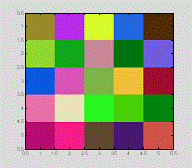
Images can also be printed to either a physical printer or a graphics file as follows. Here we are saving to a jpeg image, but the print command on it's own would send the figure to your computers' default printer.
filenames={'img 1', 'img 2', 'img3'};
image(rand(5,
5, 3));
print(filenames{i}, '-djpeg');
end
Movies
Now let's create and save a movie. Matlab has a movie function, but it only allows you to play movies in Matlab, so it's usually best to carry out one additional step and save the file as an avi. There's lots of cheap software out there (e.g. Quicktime) which you can use to convert avi to any other file type you like. In Footsteps.m we'll create a rather funky illusion discovered by Stuart Anstis of UCSD.
%
% Fixate on the red cross and observe the blue and yellow
patches.
% Whenever the grid is visible, the boxes seem to step out of
phase,
% while in reality
their movement is always parallel.
%
% Anstis SM (2003) Moving objects appear to slow down at low
contrasts.
% Neural Netw 16:933-938;
% Anstis SM (2004) Factors affecting footsteps. Vis Res
44:2171-2178;
% Thompson P (1982)
Perceived rate of movement depends on contrast. Vis Res 22:377-380
%% movie parameters
reps=2;
% number of times to repeat the movie
fps=24;
% movie frames per second
% timing parameters
tSteps=500; % must be less
than imgSize(1)-(3*stripeWidth)
altRate=200; % alternate
between gray and stripes every 200 frames
altProp=.75;
% proportion of the time use the striped background
%% background
imgSz=[600,
600];
blank=ones(imgSz); % create the gray background
stripeWidth=20;% create the
background stripes
stripes=repmat([zeros(imgSz(1), stripeWidth), ones(imgSz(1), stripeWidth)], ...
1, imgSz(2)/(2*stripeWidth));
stripes=stripes+2;
%% add fixation
cross
stripes(549:551,
525:575)=6;
stripes(525:575,
549:551)=6;
blank(549:551,
525:575)=6;
blank(525:575,
549:551)=6;
%% determine
position and size of the blue and yellow squares
boxWidth
= 2*stripeWidth;
boxHeight
= 30;
% Top, Bottom,
Left, Right
bpos=[100
100+boxHeight 20 20+boxWidth];
ypos=[200
200+boxHeight 20 20+boxWidth];
%% colormap
cmap=[
.5 .5 .5; ... % blank
.2 .2 .2; ... % stripes
.9 .9 .9; ... % stripes
.0 0 .7; ... % blue box
1 1 0; ... %
yellow box
1 0 0 ]; %
fixation cross color
% recreate the
background
if mod(t, altRate)<(altRate*altProp)
img=stripes;
else
img=blank;
end
% reposition the boxes
img(bpos(1):bpos(2),
bpos(3):bpos(4))=4;
img(ypos(1):ypos(2),
ypos(3):ypos(4))=5;
bpos(3:4)=bpos(3:4)+1;
ypos(3:4)=ypos(3:4)+1;
%image, and save a movie frame
image(img);
colormap(cmap);
axis off
F(t)=getframe;
end
close all
On each timestep we save the figure window as a movie frame. If you don't want to bother plotting it first, you can use the command im2frame.
Matlab movies are played in figure windows. To make it look pretty we are going to create a figure window that is sized to fit the movie frame and erase the axis.
% create a figure
to play the movie in that is the same size as the movie
% frame
[h,
w, p] = size(F(1).cdata); % use 1st frame to get dimensions
hf
= figure;
% resize figure
based on frame's w x h, and place at (150, 150)
set(hf, 'position', [150
150 w h]);
axis
off
% play movie, final
arguments tells movie to place the frames at bottom
% left
movie(hf,F,reps,fps,[0 0 0 0]);
The first argument to movie is the figure window handle, the next is the collection of movie frames, the number of times to repeat the movie, the frames per second and the final argument tells movie to position the frames in the bottom left corner.
Then we will write to an avi file.
%% write to an avifile
filename='Footsteps';
movie2avi(F,filename)
Warning: The frame width has been padded to be a
multiple of four as
required
by the specified codec.
> In avifile.addframe at
172
In movie2avi at 64
The quality of your movie will depend a great deal on the amount and type of compression you use. The avi movie created below will have much higher quality, but will also take up a lot more disk space (as you can check by right clicking both files and choosing "properties").
movie2avi(F,filename,
'fps', fps, 'compression', 'None', 'quality', 100);


