Chapter 5: Logical operations and some funky visual stimuli
You have actually now learned most of the basic skills you need to program 90% of most experiments. Here we are going to use some of the things we have learned to make some funky visual stimuli. This chapter is mostly revision, showing you how the skills you have learned in the previous chapter can used to create visual stimuli.
Create an m-file called SineInAperture.m
We will begin by making a sinusoidal grating.
clear all
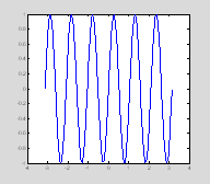
close allx=linspace(-pi, pi, 100);sf=6; % spatial freq in cycles per imagesinewave=sin(x*sf); plot(x, sinewave);
This gives us a 1-dimensional sinusoidal grating with a frequency of 6 cycles in the distance between –pi and pi. pi is a reserved variable in matlab which means that it represents the number 3.1416 without you having to define it as such. Other reserved variables are i and j). To create a 2D version of this sinusoid we will calculate the outer product of the one-dimensional sinusoid with a vector of ones.
The command close all closes all the figure windows.
close all
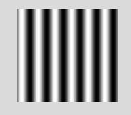
onematrix=ones(size(sinewave));sinewave2D=(onematrix'*sinewave);colormap(gray)
imagesc(sinewave2D)
axis
off;
Gratings like these are commonly used to study the visual system, partly because they are good stimuli for stimulating cells at early stages of the visual system and partly because of some mathematical properties that are discussed in Section 3.
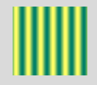
You can also look at what this sinusoid looks like with a different kind of colormap.
Now try to create a horizontal rather than a vertical grating.
Scaling images
The command imagesc scales the values in sinewave2D before plotting so as to match the colormap you are using. Default color maps have 64 rows, so imagesc rescales sinewave2D to range between 1 and 64.
If we want, we can scale the matrix ourself to match the colormap. One advantage of this is that we don't automatically use the entire contrast range of the colormap. So in the case of grayscale, the image can be low contrast instead of automatically varying between black and white.
sinewave2D varies between -1 and 1. On normal monitors, we can use up to 256 different colormap values, as is described in more detail in Section 3. So we want to rescale sinewave2D so it varies between 1-256, so the values in sinewave2D match the 256 rows in the colormap. We'll then use the image command, which doesn't do any rescaling.
scaled_sinewave2D=((sinewave2D+1)*127.5)+1;
Those parts of sinewave2D that equal -1 will be scaled to equal 1.
1
Those parts of sinewave2D that equal 0 will become 128.5
128.5000
And those parts of sinewave2D that
equal 1 will become 256
256
% rescales numbers between -1 and 1 to lie between 1
and 256
colormap(gray(256))
axis
equal
axis off
The image looks identical, but this time we are scaling it outselves rather than letting Matlab do it for us.
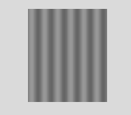
Let's make the image low contrast. If we wanted the sinewave to be 1/5 of the full contrast range (here we're assuming that we have a linear monitor which is almost certainly false, see Section 3 for details on monitor calibration) we would do the following.
scaled_sinewave2D=(((contrast.*sinewave2D)+1)*127.5)+1;
image(scaled_sinewave2D)
% rescales numbers between -1 and 1 to lie between 1
and 256
colormap(gray(256))
axis
equal
axis
off
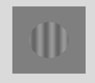
Now we are going to window this 2D sinuisoid inside a circular aperture.
for
r=1:length(x)
for c=1:length(x)
if x(r)^2+x(c)^2>rad^2
sinewave2D(r, c)=0;
end
end
end
scaled_sinewave2D=(((contrast.*sinewave2D)+1)*127.5)+1;
image(scaled_sinewave2D);
colormap(gray(256))
axis off;
So what's happening in this loop is that we are marching our way through every row and column in scaled_sinewave2D. The line x(r).^2+x(c).^2)>rad^2 is based on the equation to calculate the radius of a circle. For every point in sinewave2D we are calculating the distance to the center of the matrix to see whether that distance is greater than the radius of the desired aperture. If it is, we make that point in the image 0.
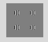
Figure 5.1 Creating a tiling of
circular apertures.
Now let's create a glorious tiling of these matrices.
imgsize=length(scaled_sinewave2D);
ntiles=2;
sep=50;
sinewave2D is 100 rows by 100 columns (imgsize). Let's suppose we wanted to create an image of 2 x 2 of these apertures (ntiles), with a 50 pixel separation between them (sep).
tilesize=(ntiles*(imgsize+sep))+sep;
tilematrix=zeros(tilesize);
The entire tile matrix will therefore need to be 350 pixels by 350 pixels (tilesize). We begin by creating a matrix that size (tilematrix) which is filled with zeros.
startpos=sep:sep+imgsize:length(tilematrix)-1;
We will then insert the apertures in four places: with the top left corner in the 50th row 50th column, 50th row 200th column, 200th row 50th column and 200th row 200th column. Because the matrix is symmetric along the rows and columns these locations can be specified with a single vector (startpos). We're going to put in the original sinewave2D matrix that varies between -1 and 1, and scale it later.
for
rtile=1:ntiles
for
ctile=1:ntiles
tilematrix(startpos(rtile):startpos(rtile)+imgsize-1, startpos(ctile):startpos(ctile)+imgsize-1)=sinewave2D;
end
end
We then go through the rows and the columns inserting sinewave2D into tilematrix. Let's think about what happens when r=1 and c=1. We will insert sinewave2D into the following position in tilematrix:
tilematrix(startpos(1):startpos(1)+imgsize-1, startpos(1):startpos(1)+imgsize-1)
Looking at this more closely you can see that this is the equivalent of tilematrix(50:149,50:149)
50
149
if you look at the length of 50:149
you will see that you have assigned a space that has100 rows and 100 columns as
being the place in tilematrix that should be
overwritten by sinewave2D.
100
If you take out the -1, you will get an error since you are trying to put a matrix that has 100 rows and 100 columns into a space that has 101 rows and 101 columns.
tilematrix(startpos(rtile):startpos(rtile)+imgsize, startpos(ctile):startpos(ctile)+imgsize)=sinewave2D;
??? Subscripted assignment dimension mismatch.
Similarly, you can't squeeze sinewave2D into a space with less than 100 rows and columns.
tilematrix(1:50, 50:149)=sinewave2D;
??? Subscripted assignment dimension mismatch.
Let's look at this final tilematrix
scaled_tilematrix=((tilematrix+1)*127.5)+1;
image(scaled_tilematrix);
colormap(gray(256))
axis
off;
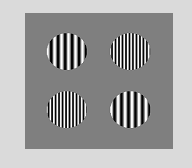
Finally, let's create a version where the apertures vary in spatial frequency.
SineInAperture2.m % information about the sinusoids
clear allclose allx=linspace(-pi, pi, 100);sf=[6 12]; % spatial freq in cycles per image
rad=3;
% creates a 100x100x2 matrix containing
two 2D apertured sinusoids
% of different
spatial frequencies.
for s=1:length(sf) sinewave=sin(x*sf(s)); onematrix=ones(size(sinewave)); sinewave2D(:, :, s)=(onematrix'*sinewave);
for r=1:length(x)
for c=1:length(x)
if x(r).^2+x(c)^2>rad^2
sinewave2D(r, c, s)=0;
end
end
end
end
% initialize
the tilematrix by filling it with zeros
imgsize=length(sinewave);
ntiles=2;
sep=50;
tilesize=(ntiles*(imgsize+sep))+sep;
tilematrix=zeros(tilesize);
startpos=sep:sep+imgsize:length(tilematrix)-1;
% do
the tiling
for
rtile=1:ntiles
for ctile=1:ntiles
if rtile==ctile
% if the 1st
tile along both the row and column direction,
% or the
2nd tile along both the row and the column direction
% then use
the first spatial frequency (6 cycles per image)
tilematrix(startpos(rtile):startpos(rtile)+imgsize-1, startpos(ctile):startpos(ctile)+imgsize-1)=sinewave2D(:, :, 1);
else
% otherwise
use the second spatial frequency (12 cycles per image)
tilematrix(startpos(rtile):startpos(rtile)+imgsize-1, startpos(ctile):startpos(ctile)+imgsize-1)=sinewave2D(:,
:, 2);
end
end
end
% image the final tilematrix
scaled_tilematrix=((tilematrix+1)*127.5)+1;
image(scaled_tilematrix);
colormap(gray(256))
axis off;
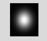
We can create a more sophisticated image by using a for loop to determine the value of a pixel rather than simply turning it into a 0. For example, if we want to calculate an image of a 2-dimensional Gaussian, we can define the values in the following nested for loop:
Gaussian1.m
%
% Method 1 of windowing a sinusoid in a Gaussian using
a nested for loop
n = 101; % size of the nxn
image of a Gaussian
Gaussian = zeros(n); % define a n x n matrix of zeros
x = linspace(-2,2,n); % define the values for x and y axes
y = linspace(-2,2,n);
for
j=1:n % columns
for i=1:n % rows
% as i and j range from 1 to n,
% x(i) and y(j) will range from -2 to 2.
% We can
then do math on x(i) and
y(j) for each pixel:
Gaussian(i,j) = exp(-x(i).^2-y(j).^2);
end
end
As the variables i and j range from 1 to 101, x(j)and
y(i) range from -2
to 2. When i=1 and j=1, which
is the top left of the image, x(j) and y(i) are both equal to one. So in this case exp(-y(i).^2-x(j).^2) = .1353.
When i=51 and j=51,
which is the center of the image, x(j) and y(i) are both equal to zero. So in this case exp(-y(i).^2-x(j).^2) = 1.
So Gaussian will have a maximum value of 1 at the center, and drop off from there.
Notice a couple of stylistic issues. First, we've defined the variable n to be the size of the image. We could have typed in the number 101 wherever n appears. But by defining n as a variable instead using the number 101, we can easily change the resolution of our picture. Try changing n to 10 and seeing what the picture looks like.
Defining numbers as variables is called soft coding (instead of hard coding). Soft coding is convenient because it allows you easily change the parameters of a program by only changing a single line. It's also easier to read provided you give your variables sensible names. A good rule is that if you use the same number more than two or three times in your program, it's a good idea to use soft coding and replace that number with a variable. (While you are a beginner it's sometimes easier to begin a program using hard coding, and then replace the hard coding with soft coding.)
% Do the usual graphics stuff to show the image
figure(1)
clf
image((255*Gaussian)+1);
colormap(gray);
axis
equal
axis
off
Because Gaussian goes between 0 and 1, when rescaling Gaussian for image we no longer need to add 1 before multiplying by the scale factor. We still need to add 1 at the end so that 0 in the Gaussian becomes 1 in the colormap.
One of the pecularities of Matlab (as compared to languages like C or Fortran) is that for loops are actually quite slow and should be avoided when possible. Nested for loops (one for loop inside another) end up being particularly slow – in the example above Matlab acually has to iterate around the second for loop n x n times (10201 times). Luckily in this case it's easy to replace the nested for loop with a command called meshgrid.
Gaussian2.m
%
% Method 2 of windowing a sinusoid in a Gaussian using
meshgrid
n = 101;
[X,Y] = meshgrid(linspace(-2,2,n));
Gaussian = exp(-X.^2-Y.^2);
image((255*Gaussian)+1);
colormap(gray(256));
axis
equal
axis
off
All this in a seven line program! Notice that there aren't any for loops either. The trick is the meshgrid command that takes in the vector ranging from -2 to 2, and returns two matrices which we've called X and Y.
Let's take a look at sizes of these two matrices X and Y.
101 101
101 101
They're both 101 by 101 matrices, where 101 is the length of the vector that was sent into meshgrid. Let's look more closely at these matrices.
imagesc(X);
colormap(gray)
axis
equal;axis off
title('X');
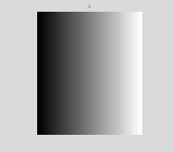
The matrix X goes from dark on the left to white on the right, with each column containing the same value. We can't see the actual values in this image, so let's let look at these values directly.
-2
X(101, 1)
-2
The first column of X is always -2.
2
2
The last column of X is always 2. X contains columns that range from -2 to 2 as we move from left to right. Now let's do the same for the matrix Y.
imagesc(Y);
colormap(gray)
axis
equal;axis off
title('Y');
-2 -2 -2 -2 -2
2 2 2 2 2
-2.0000
-1.0400
-0.0400
0.9600
2.0000
-2.0000
-1.0400
-0.0400
0.9600
2.0000
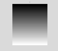
Each row in the matrix Y has the same value, and the rows range in value from -2 to 2 as we move from top to bottom.
If you think about for a bit, you'll realize that these matrices x and y are very useful for making mathematically defined images because we can now just do the math directly on these matrices without any for loops.
For example, here's a way of making a sinusoid using the X matrix of meshgrid.
n = 101;
[X,Y] = meshgrid(linspace(-pi,pi,n));
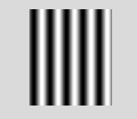
sinewave2D = sin(5*X);
figure(1)
imagesc(sinewave2D)
axis
equal;axis off;colormap(gray);
Figure 5.2 Using meshgrid to create
a 2D sinusoid.
Each element of the matrix sinewave2D is defined as the sin of 5 times each element of the matrix X. We can make a horizontally oriented grating using Y:
imagesc(horizontalGrating)
axis
equal;axis off;colormap(gray);
And you can make a Gaussian as an element-by-element function on the matrices X and Y:
Gaussian = exp(-X.^2-Y.^2);
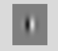
Now that we've made a sinusoidal grating and a Gaussian, we're ready to write a program MakeGabor.m that creates a Gabor by multiplying a sinusoidal grating with a Gaussian. Gabors are one the fundamental stimuli for vision research because they are a good model for a V1 receptive field.
We've added two new parameters: the parameter width determines how wide the Gaussian is, and the
parameter spatialFrequency
determins how many cycles the sinusoid makes across
the whole image. Notice how the meshgrid command makes X and
Y matrices that have values that range from –pi to pi. This way sin(spatialFrequency*x)
makes a grating that has a number of cycles equal to the parameter spatialFrequency.
Now let's use what we've learned to make a program MakeGabor.m that creates a sinusoid windowed in a Gaussian – this stimulus is called a Gabor and is also a stimulus that is regularly used to study the visual system.
% MakeGabor.m
%
% Creates a grating windowed
by a Gaussian.
clear
all;
close
all;
% define the Gabor's
parameters:
n = 201; %resolution of the image
width
= 1; %1/e half width of Gaussian
spatialFrequency
= 3;
%spatial frequency of the sinewave
carrier (cycles/image)
% Use meshgrid to create
matrices X and Y that range from -pi to pi;
[X,Y] = meshgrid(linspace(-pi,pi,n));
% Sinusoid on the matrix X makes a vertical grating.
sinusoid
= sin(spatialFrequency*X);
% Gaussian aperture:
Gaussian = exp( -(X.^2+Y.^2)/width^2);
% A Gabor is the product of the sinusoid and the
Gaussian
Gabor = sinusoid.*Gaussian;
% Show the image using the usual commands:
figure(1)
image(
(Gabor+1)*127.5); %scale Gabor between 0
and 255
axis
equal
axis
off
colormap(gray(256))
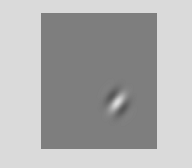
The following program, OrientedGabor.m, makes a Gabor stimulus with full flexibility over where it the Gabor is centered in the image, as well as its size, contrast, spatial frequency, orientation and phase. Play with the parameters defined at the beginning of the program to see what each one does.
% OrientedGabor.m
%
% Creates a grating windowed by a Gaussian where the following
% parameters can
vary:
% size
% contrast
% spatial frequency
% orientation
% phase
% define the Gabor's parameters:
center
= [1,1]; %[0,0] is the middle of the image, [pi,pi]
is the lower right
orientation
= pi/4; %radians (pi/4 = 45 degrees)
width
= .5; %1/e half width of Gaussian
spatialFrequency
= 6; %spatial frequency of Sinewave carrier (cycles/image)
phase
= -pi/2; %spatial phase of sinewave carrier (radians)
contrast
= 0.75; %contrast ranges from 0 to 1;
n = 201; %resolution of the image
% Use meshgrid
to define matrices X and Y that range from -pi to pi;
[X,Y] = meshgrid(linspace(-pi,pi,n));
%Create an oriented
'ramp' matrix as a linear combination of X and Y. For
%example, when
orientation = 0, cos = 1 and sin = 0 so ramp =
X. When
%orientation is
pi/2 then cos = 0; sin = 1 and ramp = Y.
ramp
= cos(orientation)*(X-center(1)) +
sin(orientation)*(Y-center(2));
% let's take a
quick look at ramp
figure(1)
imagesc(ramp)
colormap(gray(256))
axis
off
axis equal
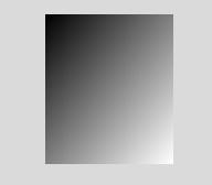
Notice how the parameter center controls the asymmetry of ramp. When center is [1, 1] the values from the top right to bottom left of ramp (shown by a purple dotted line) are -1.4. The the values in ramp that are zero (shown by a pink dotted line) lie closer to the bottom right corner. These lines of constant value are oriented diagonally because we are making a diagonal sinusoid.
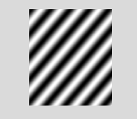
% Sinusoidal
carrier is a sinusoid on the matrix 'ramp'
sinusoid
= contrast*sin(spatialFrequency*ramp-phase);
% take a quick look at the sinusoid
figure(2)
imagesc(sinusoid)
colormap(gray(256))
axis
off
axis
equal
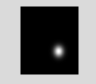
%Gaussian envelope:
Gaussian = exp(-((X-center(1)).^2+(Y-center(2)).^2)/width^2);
% take a quick look at the gaussian
figure(3)
imagesc(Gaussian)
colormap(gray(256))
axis
off
axis equal
% A Gabor is the
product of the sinusoid and the Gaussian
Gabor = sinusoid.*Gaussian;
The Gaussian is centered on the place where X-center(1)=0 and Y-center(2)=0.
%Show the image using the usual
commands:
figure(4)
image((Gabor+1)*127.5); %scale Gabor between 0 and 255
axis
equal
axis
off
colormap(gray(256));
Figure 5.2 Using meshgrid to create an oriented sinusoid.
To show this stimulus properly you need to 'calibrate' your
display so that you know exactly how much light is coming off the monitor for
each value in the color map. We'll get in to calibration later in Section 3.
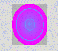
Finally, here's an example of using meshgrid to make a cool illusion. ColorIllusion.m.
% ColorIllusion.m
% creates the image of a color illusion
% the gray circles are the same
% gray, but don't look the same
close
all
[x,y]
= meshgrid(linspace(-1,1,401));
r = sqrt(x.^2+y.^2);
r(r>=.25
& r<=.3) = 0;
r(r>=.75 & r<=.8) = 0;
image((r+1)*127.5);
axis
equal
axis
off
colormap([[.7 .7 .7]; cool(256)]);
meshgrid creates two matrices - the rows of x are copies of the vector linspace(-1,1,401) (which goes from -1 to 1 in 401 steps) and the columns of y are copies of linspace(-1,1,401).
We then find points where the radius is greater than .25 and less than .3 and make those
points in the matrix 0. We then scale the matrix r between 0-255 and image it.
Remember that the inner and outer rings were set to be 0, which means that they will take the first value of the colormap. Here we fix the first value of the colormap to be gray, [0.7 0.7 0.7] and then allow the rest of the colormap to take nice funky colors. You can also try out this illusion using other colormaps like spring and hsv etc. etc. Or create your own colormap.
