Chapter 7: Sound
In this chapter we are going to describe basic methods for generating sounds. The techniques described in this chapter are useful for sounds where you don't care particularly about the response latency (the time between telling the computer to make a sound, and the moment the sound actually comes out of the speakers). You can use these simple sound commands to play beeps to warn subjects that a trial is about to begin, or to give feedback.
However sometimes it is important to be able to play back sound signals with very low onset latencies. Examples include audio experiments where subjects have to discriminate between stimuli separated by very small pauses, or audio-visual experiments where the audio stimulus must be in exact synchrony to the onset of a visual (or tactile) stimulus. Standard sound drivers and output functions as provided by Matlab are not really well suited for low latency sound playback with high timing precision and you then need to use specialized software designed for the task. More specialized sound generation is described in the third section of this book.
Basic Sound
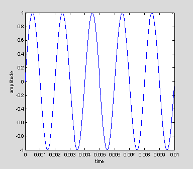
Pure tones are sine waves, the volume of the sound depends on the amplitude, and the pitch of the tone depends on the frequency.
Figure 10. Pure tones are defined by their frequency and amplitude
We are going to begin by creating a vector containing a sinusoid which we will use to generate a sound. Create an m-file called SimpleSound.m
% SimpleSound.m
%
% plays a single pure tone
clear all;
close all
freq=500; %
frequency of the tone (Hz)
dur=1.5; % duration of the tone
(seconds)
sampRate=44000;
nTimeSamples = dur*sampRate;
%number of time samples
t = linspace(0,dur,nTimeSamples);
y = sin(2*pi*freq*t);
sound(y,sampRate);
You should have heard a medium pitched tone. If you change the frequency to about 2000 Hz you should hear a higher pitched tone. The sampRate represents how finely time is sampled in the vector sent to the sound card – i.e. how many time samples per second to play the sound. Most sound cards can deal with sample rates of up to 44.1 kHz. We're using a lower sample rate here to make it easier to see the vectors in plot form.
We can look at a small sample (the first 10 milliseconds) of the signal sent to the sound card by plotting it.
indexToPlot = t<10/1000;
plot(t(indexToPlot), y(indexToPlot) );
xlabel('Time (sec)')
ylabel('Amplitude');
The amplitude of the vector here varies between -1 and 1, which represent minimum and maximum loudness. Note that there are 5 cycles over the first 10 miliseconds, which works out to be 500 cycles every 1 second (1000 miliseconds), or 500 Hz.
We can vary the loudness of the tone by simply varying the amplitude of the sinusoid.
ramp=linspace(0, 1, nTimeSamples);
figure(2)
plot(t, ramp, 'r')
xlabel('Time (sec)')
ylabel('amplitude envelope')
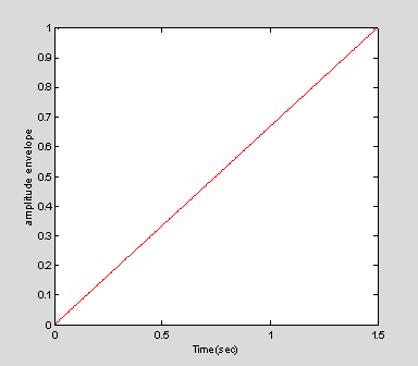
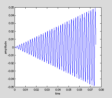
The variable ramp varies linearly from zero to one over 1.5 s. We can then simply multiply the sinusoid by the ramp to modulate the volume over time. In cases like this the ramp is often called an envelope. Here we again plot the 75 milliseconds of the signal, and you can see that the volume is gradually and linearly increasing. In fact the volume continues to increase throughout the full 1.5 s, as described by the envelope of the ramp.
sound(y2, sampRate);
plot(t(1:round(nTimeSamples/20)), y2(1:round(nTimeSamples/20)));
xlabel('time')
ylabel('amplitude')
Now let's play with creating a scale of tones. Create another m-file called PlayTones.m
% PlayTones.m
% plays a scale using the
command sound
%
% written by Geoff Boynton
May 2007
freqC =
278.4375; % Frequency of midle C (Hz) (called 'C4')
numNotes=13; %
number of notes (13 notes = one octave (C to C))
noteNumbers = [0:(numNotes-1)];
whiteKeys = [1,3,5,6,8,10,12,13]; %white keys on piano (key of C)
% Frequencies of
subsequent notes on the 12-tone scale
% are obtained by
multiplying the previous frequency by
% 2^(1/12).
% Example: freqD = freqC*(2^(1/12))
% freqE
= freqD*(2^(1/12)) = freqC*(2^(2/12))...
multFac = 2.^(noteNumbers/12);
allFreqs = freqC*multFac;
% Now,
let's make sound waves containing tones for each note
dur = .8; %duration of the tone (Seconds)
ISI = 1; %time between the
start of each note (Seconds)
sampRate = 8192; % Sampling rate for sound (Hz)
nTimeSamples = dur*sampRate; %
number of time samples
t = linspace(0,dur,nTimeSamples);
tic
for i=1:length(whiteKeys)
freq = allFreqs(whiteKeys(i));
y= sin(2*pi*freq*t);
sound(y,sampRate);
while toc<i*ISI
;
end % end of the
while loop
end
tic starts a stopwatch. toc measures the time since the stopwatch started. Try the following
Elapsed time is 2.946064 seconds.
Elapsed time is 6.216524 seconds.
Elapsed time is 9.603302 seconds.
You can see how the time values of toc gradually increase. They will continue to increase until you call tic again, which will restart the stopwatch.
Here we are using tic and toc inside something called a while loop. A while loop tells Matlab to repeat the content of the loop until the expression following the while (toc<i*ISI) is false. In this case the content of the loop is just a semicolon, so Matlab just spins around the loop doing nothing until the time that has elapsed since tic is greater than i*ISI. So the first time through the while loop Matlab waits until 1 second has gone by since tic was called, the second time Matlab waits until 2 seconds have gone by, and so on. This adds an acoustically pleasing pause in between each note.
Stereo
Now let's play these tones in stereo. To control the left and right speakers separately sound requires an n x 2 (two column) matrix instead of a simple 1d vector. Replace the last lines of PlayTones.m with the following code, and listen to it using headphones so you can hear the stereo. You should hear the tones alternate between the left and right speakers.
for i=1:length(whiteKeys)
freq
= allFreqs(whiteKeys(i));
y= sin(2*pi*freq*t)';
sndmat=repmat(y,
1, 2);
if mod(i, 2)==0
sndmat(:, 1)=0;
else
sndmat(:, 2)=0;
end
sound(sndmat, sampRate);
while toc<i*ISI
;
end %
end of the while loop
end
We've used a couple of new tricks in this code. One is the command repmat. Repmat replicates a vector or matrix. It takes as its first input argument the vector or matrix to be replicated, its second argument is the number of times you want to replicate that vector or matrix along the row dimension and its third argument is the number of times you want to repeat it along the column direction.
x=[1 2 3];
repmat(x, 1, 3)
1 2 3 1 2 3 1 2 3
1 2
3
1 2
3
1 2 3
1 2
3 1 2
3
1 2
3 1 2
3
1 2 3 1 2 3
And here's an example of using repmat on a 2D matrix.
x=[1 2 3; 4 5 6]
repmat(x, 1, 2)
1 2
3
4 5
6
ans
=
1 2
3 1 2
3
4 5 6 4 5 6
In the code above we replicated the vector y along the y direction to create a n x 2 matrix. We then replaced either the first or the second column with zeros with the commands sndmat(:, 1)=0; and sndmat(:, 2)=0; That is what made the sound come out of either the left or the right speaker - the values in column 1 are assigned to the left speaker, and those in column 2 to the right speaker.
mod calculates the modulus (remainder) after division.
1
2
We used the statement if mod(i, 2)==0 to detirmine whether it was the left or right speaker that was zero-ed out. When i is an even number mod(i, 2)==0 is true. When i was an odd number it is false. So we alternate between blanking out the left and the right speakers as i alternates between being even and odd.
MovingNoise.m
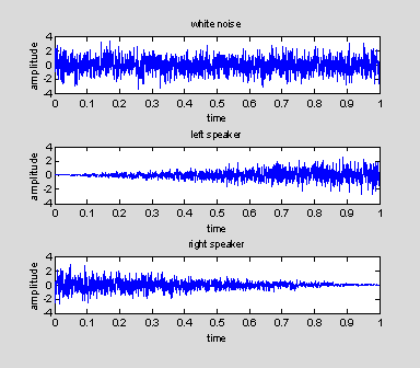
Here's a final example of creating sound in Matlab– this time we're going to make a white noise stimulus that fades from left to right. We're going to use a very low sampling rate here so you can visually see what is happening. If you were using such a stimulus in an experiment you should use a much higher sampling rate.
% MovingNoise.m
% a white noise stimulus that moves from left to right and back again.
close all
dur=1; %
duration of the tone
sampRate=2000;
nTimeSamples = dur*sampRate;
%number of time samples
t = linspace(0,dur,nTimeSamples);
ramp=linspace(0, 1, nTimeSamples);
y=randn(1, nTimeSamples); %
create a white noise vector
rampednoise1=[y.*ramp]'; % transpose so a single column
y=randn(1, nTimeSamples);
rampednoise2=flipud([y.*(ramp)]');
soundsc([rampednoise1;rampednoise2],sampRate);
plot(t, y);
xlabel('time'); ylabel('amplitude');
axis([0 1 -4 4]);
title('white noise');
subplot(3, 1, 2);
plot(t, rampednoise1);
xlabel('time'); ylabel('amplitude');
axis([0 1 -4 4]);
title('left speaker');
subplot(3, 1, 3);
plot(t, rampednoise2);
xlabel('time'); ylabel('amplitude');
axis([0 1 -4 4]);
title('right speaker');
The amplitude of the white noise gradually increases in the left speaker and decreases in the right speaker, giving the impression that the noise is moving in space. There are a few new commands here.
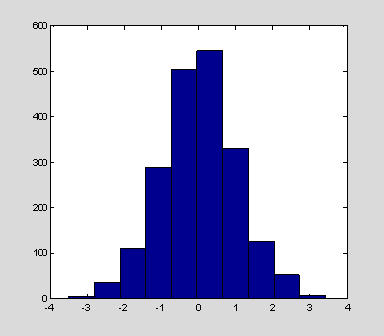
randn provides a list of random numbers that are normally distributed with 0 mean and a variance of 1. If you take a histogram (hist) of the values in y, you will get something that looks like a normal distribution with zero mean and unit variance. A stimulus like this is called white noise. White noise is often used as a way of masking auditory stimuli for mathematical reasons we'll discuss in Section 3. For example, in an experiment where you measure the ability of a subject to disciminate vowel sounds, if you wanted to make the task more difficult you might add white noise to the vowel sound.
clf
hist(y)
flipud flips the vector y vertically (i.e. flips along the row dimension). fliplr will flip a vector horizontally (i.e. flips along the column direction). Here's a few simple examples of how they work.
x=[1 2 3]
fliplr(x)
1 2
3
ans
=
3 2 1
1 2 3
This does nothing because x only has a single row. But try the following:
x=[ 1 2 3; 4 5 6]
flipud(x)
1 2
3
4 5
6
ans
=
4 5
6
1 2 3
3 2
1
6 5 4
Note that in the code above we transposed y to be a column vector, (i.e. a vector restricted to a single column) and then flipped the rows vertically. We could instead have flipped ramp horizontally while it was still a row vector, (i.e. a vector restricted to a single row) multiplied it by y, and done a transpose on the final product. We would have ended up with the same thing.
y=randn(1, nTimeSamples);
rampednoise2=([y.*fliplr(ramp)]');
Finally, we use the command soundsc instead of sound. This is because the vectors rampednoise1 and rampednoise2 have values that range beyond -1 to 1. soundsc automatically scales our input to vary between -1 and 1 (we'll discuss scaling noise in more detail later in this chapter). sound clips values greater than 1 and less than -1 to +/-1 – which will seriously distort your sound, as you can easily see by comparing what this white noise sounds like using both commands.
soundsc([rampednoise1;rampednoise2],sampRate);
sound([rampednoise1;rampednoise2],sampRate);
Saving and loading sound files.
You may want to save the tones you used so you can (for example) use them in a talk to an audience, or use pre-recorded clips of sound. Here’s how to convert vectors to and from wav files using wavread and wavwrite.
There’s a bunch of cheap software (~$20) on the web that
will help you convert any kind of audio file you like into wav files. Or, if
you go to the user community part of the Mathworks
website (http://www.mathworks.com/matlabcentral/)
and search (e.g. using the search term mp3) you can probably find free Matlab code that will do the conversion for you.
ToneInNoise.m
% ToneInNoise
%
% An
example of creating a tone masked by white noise
% Also
provides an example of reading and writing wave files
%
% written by if & gmb 5/2007
We’ll start by making a vector for a tone masked by white noise
close all
dur=1; %
duration of the tone
sampRate=44.1*1000; % using highest sample rate
nTimeSamples = dur*sampRate;
%number of time samples
% create white noise
vector
noise=randn(1, nTimeSamples); %
create a white noise vector
% create tone
t = linspace(0,dur,nTimeSamples);
freqC =
278.4375; %Frequency of midle C (Hz) (called 'C4')
tone = sin(2*pi*freqC*t);
Up to now we've allowed the loudness of our stimuli to be determined by soundsc, so we've always used the maximum volume range of the speakers. Here we're going to control the volume of the noise and the tone separately.
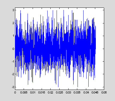
If we look at noise, the range of values is much larger than -1 to 1, and the maximum and minimum values depend on the numbers thrown up by randn. As you might expect, mostly they vary between -2 and 2, but some values are greater than +/- 3.
plot(t(1:2000), noise(1:2000));
axis([0 .05 -3.2 3.2])
min(noise)
4.1563
ans
=
-4.0453
We're going begin to "clipping" the noise, by setting all values above 3 standard deviations to be 3 (as you recall, the noise had a single standard deviation of 1). find gives you a list of all the values in noise that are greater than 3. We'll then use ind to replace those values with 3.
ind
Columns 1
through 8
138 939 1038 1210 1418 1694 2806 3019
Columns 9
through 16
3490 4189 5309 6370 6675 10237 10692 11424
Columns 17
through 24
11548 11549 12679 14095 14232 15214 15915 16557
Columns 25
through 32
17718 18282 18316 18762 19263
19342 19530 20315
Columns 33
through 40
20569 20638 21839 22032 22460 22634 23302 23631
Columns 41
through 48
24246 25994 27362 27859 28643 29513
29711 30227
Columns 49
through 56
31629 32424 33243 33357 34213 34644 36757 38929
Columns 57
through 63
39191 39725 41228 41729 42175 42385 42918
1 63
1 44100
Size gives us (surprise!) the size of any variable. As you can see we've replaced just over 1% of our time points. This isn't too bad and shouldn't distort our signal too badly. We'll do the same for values less than -3.
noise(ind)=-3;
Let's look again at noise. You can see that values are no longer are outside the range of +/- 3.
min(noise)
3
ans
=
-3
plot(t(1:2000), noise(1:2000));
axis([0 .05 -3.2 3.2])
Now let's add noise and signal together, while scaling the amplitude of each one. Remember that it's the final signal that can't exceed +/- 1. Given that the noise varies between +/-3 and the tone varies between +/- 1 this means that the following must be true
toneamp+3*noiseamp<=1 for the signal to be in range. See what happens as you change the values of noiseamp and toneamp. You're interested in what noisetone sounds like as these values vary, as well as simply finding out which values are acceptable to the program. Adding checks and warnings like these is a large part of good programming.
% add the vectors together
% amplitudes of noise and signal
noiseamp=.25; % scale the amplitude of the noise as
compared to the tone
toneamp=0.25;
if toneamp+3*noiseamp>1
disp('warning,
noise out of range')
else
noisetone=(toneamp.*tone)+(noiseamp*noise);
sound(noisetone,sampRate);
end
Finally, let's write this sound to a wave file.
wavwrite(noisetone,sampRate, 'mytone');
disp(['tone has been written to directory ', pwd])
tone has been written to directory C:\Program Files\MATLAB\R2007b
Now we’ll read the wave file back into Matlab and play it. When we load in this wavefile, the first output argument is what we are going to call the sound vector, the second argument is the sampling frequency. So M should be identical to noisetone, and FS should be identical to sampRate.
[M,FS]=wavread('mytone.wav');
sound(M, FS);
44100
44100
-0.1929
0.0204
0.1432
-0.1678
0.5986
0.1762
0.2294
0.0914
0.2051
0.3545
Columns 1
through 9
-0.1929 0.0204
0.1432 -0.1678 0.5986
0.1762 0.2294 0.0914
0.2051
Column 10
0.3545
M is a column vector and noisetone a row vector, but otherwise they are identical. If you send a 1D vector to sound it will automatically flip it to be a column vector, which is why sound treats both these vectors as being identical despite being oriented differently.
