Homework 10 Solutions
Section 7.1
Page 472, #2
|
Response |
Observed |
Expected |
|
A.
Limited advancement |
78 |
82 |
|
B.
Lack of recognition |
52 |
50 |
|
C.
Low pay/benefits |
30 |
30 |
|
D.
Unhappy with management |
25 |
20 |
|
E. Bored/Don’t know |
15 |
18 |
(a)
H0:
The distribution of reasons is 41% A, 25% B, 15% C, 10% D, and 9% E.
H a:
The distribution differs from the expected.
(b) 
(c) ![]()
(d)
Fail
to reject H0. Not enough
evidence to reject the claim that the distributions are the same.
Page 475. #12
Step 1: Calculate the sample mean of the distribution
![]() , where x is the midpoint of each class
, where x is the midpoint of each class
![]()
Step
2:
Calculate the sample standard deviation

Step 3: Calculate z-scores for the upper
and lower bounds of each of the classes
|
Lower Bound |
Upper Bound |
Zlower |
Zupper |
|
50.5 |
60.5 |
|
|
|
60.5 |
70.5 |
|
|
|
70.5 |
80.5 |
|
|
|
80.5 |
90.5 |
|
|
|
90.5 |
100.5 |
|
|
Step
3:
Calculate areas between each of the bounds
|
Zlower |
Area to left of Zlower |
Zupper |
Area to left of Zupper |
Area between classes = area(Zupper) –
area (Zlower) |
|
-2.47 |
.0068 |
-1.45 |
.0735 |
.0667 |
|
-1.45 |
.0735 |
-0.44 |
.3300 |
.2565 |
|
-0.44 |
.3300 |
0.58 |
.7190 |
.3890 |
|
0.58 |
.7190 |
1.60 |
.9452 |
.2262 |
|
1.60 |
.9452 |
2.62 |
.9956 |
.0504 |
Step
4:
Calculate Expected Frequencies for each class by multiplying the area in each
class times the total number of test scores
|
Class |
Area |
Expected
Frequency |
|
50.5
– 60.5 |
.0667 |
(400)(.0067)
= 26.68 |
|
60.5
– 70.5 |
.2565 |
(400)(.2565)
= 102.6 |
|
70.5
– 80.5 |
.3890 |
(400)(.3890)
= 155.60 |
|
80.5
– 90.5 |
.2262 |
(400)(.2262)
= 90.48 |
|
90.5
– 100.5 |
.0504 |
(400)(.0504)
= 20.16 |
Step
5:
Calculate ((O-E)2)/E
|
Class |
Observed
Frequency |
Expected
Frequency |
|
|
50.5
– 60.5 |
28 |
26.68 |
|
|
60.5
– 70.5 |
106 |
102.6 |
|
|
70.5
– 80.5 |
151 |
155.60 |
|
|
80.5
– 90.5 |
97 |
90.48 |
|
|
90.5
– 100.5 |
18 |
20.16 |
|
Step 6: Calculate test statistic
![]()
Step
7:
Calculate the degrees of freedom and critical value
1.
Degrees of Freedom
(a) The text
equated the sample mean and sample standard deviation with the population
mean
and standard deviation. In this case,
the degrees of freedom is k-1 = 4.
With
k=4, α = .05, χ2=9.488.
(b) Perhaps more correct is to subtract a degree of
freedom for each of the sample
statistics calculated. In that
case, the degrees of freedom are k-1-2 = 2, and χ2=5.991.
Step
8: Make
your decision.
χ2
< χc2, so fail to reject the null hypothesis that
the 400 test scores are normally distributed.
It can be concluded that the test scores are normally distributed.
Section 10.2
Page 483, #6
|
|
Treatment
|
|
|
Result
|
Drug |
Placebo |
totals |
|
Impovement |
20 (18) |
19 (21) |
39 |
|
No Change |
10 (12) |
16 (14) |
26 |
|
totals |
30 |
35 |
65 |
(a) H0:
The treatment is independent of the result.
H a:
The treatment is not independent of the result.
(b) df = (r – 1)(c – 1) = (2 – 1)(2 – 1) = 1
![]()
(c) ![]()
(d)
Fail
to reject the null hypothesis. There is
not enough evidence to support the claim that the treatment and result are
dependent. I would not recommend the
drug.
Page 485, #12
H0: The proportions are equal.
H a:
At least one of the proportions is different from the others.
|
|
Treatment
|
|
|
Result
|
Drug |
Placebo |
totals |
|
Impovement |
39 (31.66) |
25 (32.34) |
64 |
|
No Change |
54 (61.34) |
70 (62.66) |
124 |
|
totals |
93 |
95 |
188 |
![]()
![]()
Reject H0. Recommend the drug.
Section 10.3
Page 494, #16
(a) H0: s1 = s2 (claim)
H a:
s1
≠ s2
(b) F0 = 4.77
(c) ![]()
(d)
Fail
to reject H0. There is not
enough evidence to refute the claim that the population variances are equal.
Page 495, #22

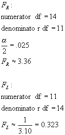
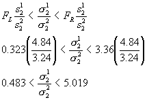
95% Confidence Interval:
