Homework 4
Solutions
Page 159 #12
x is discrete. The number of rainy days has a finite, countable number of outcomes.
Page 160 #18
0 ≤ P(x) ≤ 1 for all P(x)
Σ P(x) = .005 + .435 + .555 + .206 = 1.201
Since the probabilities do not sum to 1, this is not a probability distribution.
Page 161 #26
(a)
|
x |
P(x) |
x ∙ P(x) |
x-m |
P(x) ∙(
x-m)2 |
|
0 |
.1521 |
0 |
-1.8655 |
0.52913 |
|
1 |
.2924 |
.2924 |
-0.8655 |
0.21903 |
|
2 |
.2485 |
.4971 |
0.1345 |
0.0045 |
|
3 |
.1784 |
.5352 |
1.1345 |
0.22957 |
|
4 |
.1023 |
.4092 |
2.1345 |
0.46627 |
|
5 |
.0263 |
.1315 |
3.1345 |
0.25856 |
Total |
1 |
1.8655 |
|
1.70706 |
(b) μ = 1.8655
(c) σ2 = 1.7071
(d) σ = 1.3065
(e) The mean number of accidents per student is 1.8655, with a standard deviation of 1.3065accidents.
Page 162 #28
|
x |
P(x) |
x ∙ P(x) |
x-m |
(x-m)2 |
P(x) ∙(
x-m)2 |
|
0 |
.994 |
0 |
270 |
72,900 |
72,462.6 |
|
-30000 |
.004 |
-120 |
-29730 |
883,872,900 |
3,535,491.6 |
|
-60000 |
.001 |
-60 |
-59730 |
3,567,672,900 |
3,567,672.9 |
|
-90000 |
.001 |
-90 |
-89730 |
8,051,472,900 |
8,051,472.9 |
|
Total |
1 |
-270 |
|
|
15,227,100 |
(a) μ = -270
(b) σ2 = 15,227,100
(c) σ = 3902.192
(d) E(x) = -270
(e) The insurance company should expect to pay $270 for each claim, with a standard deviation of $3902.19.
Page 163 #32 (Use probabilities from Ex. 26 and
substitute “accidents” for “computers”)
|
X |
students |
P(x) |
|
0 |
260 |
0.152047 |
|
1 |
500 |
0.292398 |
|
2 |
425 |
0.248538 |
|
3 |
305 |
0.178363 |
|
4 |
175 |
0.102339 |
|
5 |
45 |
0.026316 |
Total |
1710 |
1 |
(a) P(no
accidents) = ![]()
(b) P(at least one accident) = 1 – P(no accidents) = 1 -.1521 =.8479
(c) P(between 1 and 3 accidents) = P(1
accident) + P(2 accidents) + P(3 accidents) = .292398
+ .248538 + .178363 = .719
Page 163 #34
Note that you need to account for the $4 that you spend on the ticket. So, if you win the $3150, you really only gain $3146, since you paid $4 for the ticket.
|
Gain, x |
$3146 |
$446 |
$21 |
-$4 |
|
Probability, P(x) |
1/5000 |
1/5000 |
15/5000 |
4983/5000 |
![]()
Page 173 #4
This is a binomial experiment. “Success” is that a person does not buy something, n is 15, and p is .70. The possible values of x are 0, 1, 2, . . . , 15.
You can define success however you want. So, it is okay to have a success defined as NOT buying something.
Page 174 #8
(a) ![]()
(b) 
(c) ![]()
Page 175 #14
|
x |
P(x) |
|
0 |
|
|
1 |
|
|
2 |
|
|
3 |
|
|
4 |
|
|
5 |
|

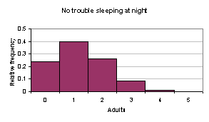
(c) μ = np = 5 x .25 = 1.25
(d) σ2 = npq = .9375
(e)
σ = ![]() .968246
.968246
(f) The average number of adults, out of 5, that say they have no trouble sleeping at night is 1.25, with a standard deviation of .968246. It would be unusual to find 5 out of 5 adults that said they had no trouble sleeping at night.
Page 176 #20 (BONUS)
![]()
Page 182 #2
Since we are given a mean, and asked to find the probability of a certain number of occurrences in an interval of time, the Poisson distribution is appropriate to answer this question.
Page 182 #4
If we think of “answering yes” as a success, with a probability of .40, then the binomial distribution is appropriate here, with the number of trials equal to the number of adults surveyed.
Page 183 #12
(a) ![]()
(b) ![]()
(c) ![]()
Page 184 #18
(a) ![]()
(b) To use the Poisson distribution to approximate the binomial distribution, you must first approximate m with np:
μ = np = 6.5
![]()
Note that the answers in (a) and (b) are very similar. In this case, the Poisson approximated the binomial well.