SMARTPsych SPSS
Tutorial
Correlation and
Regression
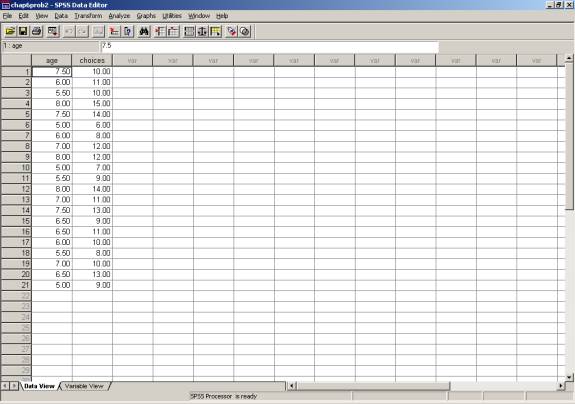
To begin, here is a data set from Roger Kirk’s Statistics: An Introduction (Chapter 6, problem #2). This experiment investigates gender-typed behavior of children as a function of their age. Enter the data as follows (also on p. 212 if you have the text). Be sure to label the variables (“age” and “choices” are used here).
Next, let’s construct a scatterplot so that we can visually inspect the data. To do this, go to GRAPHS / SCATTER. The following dialog box will appear:
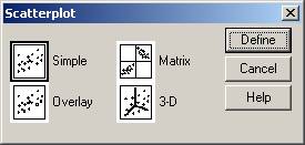
Select that you want the ‘simple’ scatterplot and choose ‘define.’ (If you are interested, you may want to inspect the matrix or 3-D scatterplot functions for your use in the future).
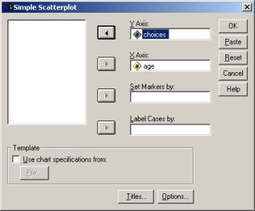
Using the convention that you place your dependent variable along the y axis and the independent variable along the x axis, select the appropriate choices to correspond to the dialog box below:
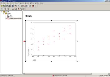
Once you hit ‘OK,’ an output window will open containing your scatterplot. At this point, you might compute the regression constants and draw a line of best fit to the data if you were doing it by hand. In SPSS, though, you’re just a few clicks away from the line of best fit! Here’s how to do it:
|
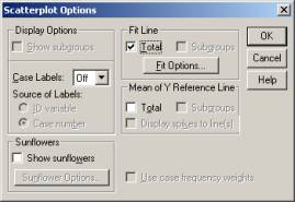
1. Double-click on your scatterplot to open the SPSS chart editor. 2. Once the chart editor is open, double-click anywhere inside the plot area, except for on the data points. 3. The dialog box below will open. Select that you want ‘Fit Line’ to be Total. In SPSS, the default is for the fit line to be based on the linear regression equation predicting y from x. |
|
Now, to find out the strength of this linear relationship, you may use either the correlation or the regression command in SPSS. In this example, both will be used, but you should know that all of the information in the correlation command can be obtained through regression. The instances in which you may want to use correlation only are:
1) You are not interested in predicting one value from the other; you only want to know the strength of the relationship.
2) You want a correlation coefficient (r) other than Pearson, such as Spearman’s rank coefficient.
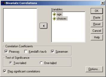
To run the correlation command in SPSS, select ANALYZE / CORRELATE / BIVARIATE. In your student version of SPSS, the ‘analyze’ command in the menu is replaced with a ‘statistics’ command. The ‘bivariate correlations’ dialog box shows all the variables in your data set on the left, and you should select the variables that you want to correlate and move them to the right. I’ve selected both ‘Pearson’ and ‘Spearman’ correlation coefficients here to show you that you can do both; these data are most appropriate for the Pearson r.
The output that you will get has several important parts, which are identified below:
The value .824 is
your Pearson r for this problem.
![]()
Your output is essentially a grid (matrix) of correlations. If you had three variables that you were correlating, you would get a 3 x 3 matrix of r values. Each box in the matrix gives you the r value, the significance (these values we will discuss in much greater detail in the future), and the N, or sample size for each correlation.
Also notice in your correlation output that the diagonal is composed of each variable correlated with itself (thus, r is a perfect positive correlation for these boxes).
You may notice that your Spearman r (rho) for this data set is equal to the Pearson r; this will not always be the case. The table with these values is labeled as a ‘nonparametric correlation;’ these will also be discussed in the future.
REGRESSION
Now that you are familiar with the correlation command, the following steps will show you how to get this information using the regression command in SPSS. First, choose ANALYZE / REGRESSION / LINEAR. The following dialog box will appear:
Your IV for this experiment is the child’s age. Your DV for this experiment is the number of choices.
![]()
![]()
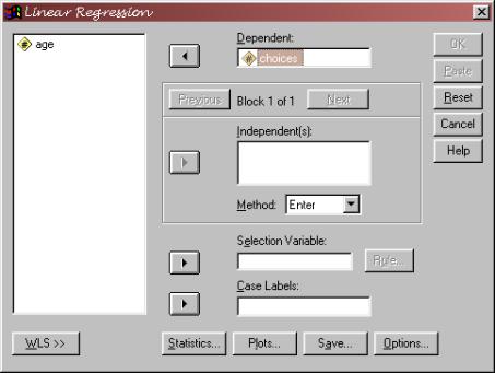
You want to select your dependent and independent variables. In the independent(s) box, notice that you can enter more than one variable. You can also choose different methods for entering these variables, and you can enter them in ‘blocks.’ Although we only have done regression analyses in which one independent variable is used to predict scores on a dependent variable, multiple regression
involves using more than one independent variable. In doing this, you would hope to improve your ability to predict dependent variable scores (increase your r squared) with the additional information gained by more than one independent variable. For example, here you may also have data on the choices that these children’s siblings make regarding gender-appropriate toys. If this is believed to influence the choices made by kids in your sample, you may want to include it as a second independent variable that enters into your regression equation.
For now, though, we’re just using simple linear regression.
Click on OK, and you should get the output that is on the next page.
This simply tells you which IVs were entered into the
regression model.
![]()
The standard
error of the estimate here is not the same value as the SY·X.
that you compute. If computing by
hand, you would get 1.328. SPSS is
slightly off because it is using the estimated standard deviations of the
populations, not the standard deviations of x and y, to compute this. The SPSS formula has n-2 in the
denominator, rather than n (minus 2 because it estimates two parameters in
doing this). To get the SY·X
value you computed, you need to multiply the SPSS value by the square root
of (n-2)/n.
![]()
![]()
![]()
Note that this is your Pearson r that you obtained
through the correlation command.
You also get R square. You
can see that the regression command is more powerful and provides more
information than the correlation command.
The ANOVA is a new concept that you will
learn about before long. Essentially,
the ANOVA (analysis of variance) is based on the regression model, and is also
a way of determining how the independent variable may explain variance in the
dependent variable.
This significance
value is the same as the significance of your Pearson r when you ran the
correlation command.![]()
![]()
Notice that in
the Unstandardized coefficients column, you have the two values used to
compute the regression line. The
slope, bY·X, is listed as the B for the variable age, and aY·X
is listed as the B for the “constant.” Don’t get confused by the notation here; your B values are
your regression coefficients.
Your regression line, taken from the coefficients table, is Yi’ = -1.964 + 1.929Xi
There are many other interesting relationships among the parts of this output. For example, the t value (a t-test of your coefficients’ ability to explain variance in your DV) in the coefficients table is the square root of the F value in your ANOVA table. OK, so don’t worry about these things now, but know that in the future, you will have a much more comprehensive understanding of all of this information and the interrelationships herein.
ASSIGNMENT
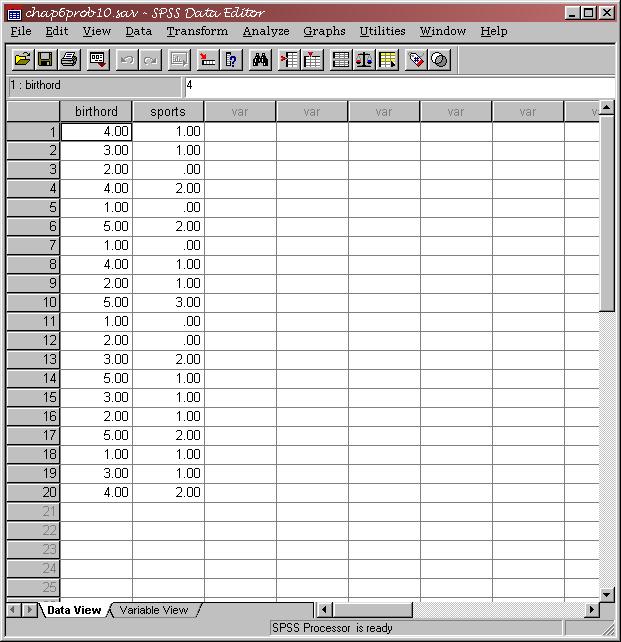
Now that you know how to do the correlation and regression commands in SPSS, use the data in Kirk’s chapter 6, problem #10 (the relationship between birth order and number of dangerous sports, p. 213) to do the following:
Run a regression that predicts number of dangerous sports from birth order, and label the following in your output:
1) The correlation coefficient r for the relationship between the two variables.
2) The standard error of estimate in predicting Y from X. ALSO transform this value to indicate what you would have obtained if you calculated SY·X by hand.
3) Regression constants, bY·X and aY·X
4) Circle the independent variable and draw a rectangle around the dependent variable (the names should be in your printout in a couple of places.
The data for this problem are shown in SPSS below.