Tutorial 3.0 - GIS Basics
Something basic about GIS (Microsoft Powerpoint)
In this exercise you will obtain GIS data from the internet, organize it in ArcCatalog, and view both spatial and attribute data in ArcMap. The purpose of this exercise is mainly to introduce you to the programs and interface of the ArcGIS platform and to the WAGDA site, where you will be obtaining most of your data for this course.
PART A. DATA ACQUISITION
- The data you will be using in this exercise (and throughout the course) comes from the Washington State Geospatial Data Archive (WAGDA). Open the web site by clicking on the following link: http://wagda.lib.washington.edu.
- At the WAGDA web site, click on Download Data Online, then on the quick link to City data for the Pacific Northwest. Scroll to the bottom of the page and click on the City of Seattle link (you'll need to enter your UW NetID at this stage and agree to the Data Use Policy). This brings you to the main page for downloading City of Seattle geospatial data.
- Download the following four files to a working directory (such as D:\documents\
): - Under the subheading Administratice / City Boundaries, download:
- Municipal Boundaries (munibond.zip)
- Under the subheading Property and Survey, download:
- Building Outlines (bldg.zip) and
- Parcel Boundaries Delineated by King County (parcel.zip).
- Under the subheading Street Network and Geocoding, download:
- Street Network (snd.zip)
- Under the subheading Transportation Data (of King County GIS data) download:
- Metro Bus Stops (Busstop.zip)
- Under the subheading Administratice / City Boundaries, download:
- These files are zipped, so you'll need to open each of them in turn in WinZip and click the Extract button to place the uncompressed files in your working directory:
- Find the downloaded zip file, right-click on it, and choose Extract to....
- In the dialog box that appears, navigate through the directory tree under Folders/drives to find your working directory, then click Extract.
PART B. FILE ORGANIZATION
The first thing you'll need to do with ArcGIS is to use ArcCatalog to establish a connection to your working directory. The ArcGIS file system does not automatically provide access to the full Windows file system, so whenever you start a new working directory, you'll need to explicitly create a connection to it.
- In the Start menu, open the Programs submenu, then choose the subdirectory ArcGIS and select ArcCatalog.
- Once ArcCatalog has opened, find and click the Connect to Folder button on the main toolbar:

- In the dialog box that appears, navigate to your working directory (should be something like this: Desktop \ Computer \ Local Disk (D:) \ Documents \
), then click OK.
- Now let's look at the ArcCatalog interface. The left portion shows a directory tree, listing all connections that have been made, all under the top-level directory called Catalog. Notice that your working directory now appears in this directory tree.
- Open your working directory by double-clicking on it, and inspect its contents to be sure that all five of the layers you downloaded have appeared. Notice that the five layers have three different icons associated with them. The busstop layer's icon indicates a point layer, the snd layer's icon indicates a polyline layer, and the icon next to boundary, parcel and bldg indicates a polygon layer.
The right portion of the ArcCatalog interface shows the contents, preview, or metadata for whatever is currently selected in the directory tree at the left. While your working directory is selected, you should see the four layers you download, along with the type for each (they should all be Shapefiles). This area allows you to quickly inspect data files one-by-one before adding them to an ArcMap project.
- Now select the "snd" layer in your directory tree. You'll see the right side change to a large icon indicating this is a shapefile with polyline data. Click on the Preview tab to look at the spatial data. You'll now see a map of all of the principal transit routes in Seattle. At the bottom of the preview, change the drop-down box from Geography to Table and scroll across to see what kinds of attribute data are included in this layer.
- Select "busstop" layer and repeat the previous step. How many bus stops can you find in the attribute table (look at table record)?
PART C. VIEWING MAP DATA
Next, you will begin an ArcMap project. ArcMap is the program in which you can view, edit, and manipulate spatial data layers in detail, as well as prepare maps for output.
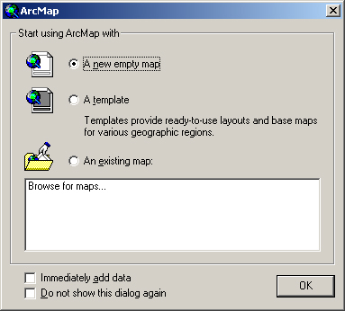
- Open ArcMap either through the Start menu or by clicking on the Launch ArcMap button in ArcCatalog:

Choose Start using ArcMap with "A new empty map"
- Once ArcMap has opened, add all four of your data layers into ArcMap, first click on the Add Data button in the main toolbar:

- In the Look in drop-down box, navigate to the connection to your working directory. Then highlight all four of your data layers by clicking the first one, holding down the Shift key, and clicking on the last one, then click Add.
You now may (or may NOT) see a dialog window that tells you one or more layers is missing Spatial Reference Information. Just hit OK.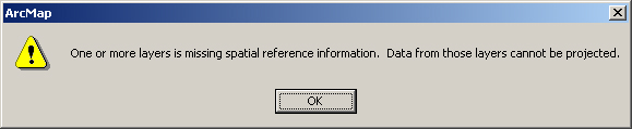
You should now see how the spatial data layers are listed in both the left and right portions of the ArcMap interface. At left you see what is called the Table of Contents, which is simlar to a map legend in that it lists the four layers and shows the symbology used to represent each layer on the map. At right, you see the map itself, with bus stops on top, transit routes beneath them, and parcels and buildings in the background.
- Let's start navigating around Seattle now. Zoom in by first clicking on the Zoom In tool:

then by clicking on the map and drawing a box around the area you want to zoom in on. Try this by zooming in on the University District.- (Tip: if the map looks incomplete and you can't find the U District, you may have interrupted ArcMap by clicking on the map while it was still drawing. To refresh the view, hit the F5 key on your keyboard and wait for it to finish drawing.)
- (Tip: if the map looks incomplete and you can't find the U District, you may have interrupted ArcMap by clicking on the map while it was still drawing. To refresh the view, hit the F5 key on your keyboard and wait for it to finish drawing.)
- You may notice that there are no buildings shown on the University of Washington campus. If this is so, it is probably because of the order of your layers in the Table of Contents. In the Table of Contents, layers at the bottom of the list are drawn first, then layers above are drawn on top, so the lowest layers can get covered up by the higher layers. If the bldg layer is at the bottom, click on it and drag it upward until a black horizontal line appears just above the parcel layer, then let go of the mouse button.
- You should now see building outlines of all of the campus buildings. Continue zooming until you can tell where Gould Hall is but you can still see its vicinity. You can continue to use the Zoom In tool, but you may also need the Zoom Out tool (
 ) to back out again or the Pan tool (
 ) to navigate laterally around the map. You should end up with a view something like this (but your colors will differ):
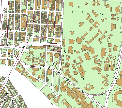
- Next, let's change the symbology of some of our layers. The easiest way to change symbology is to simply click on the symbol in the Table of Contents. Click on the symbol for the busstop layer.
- You'll see a long list of basic symbols, but nothing particurly good for bus stops. To add some options, click on the More Symbols button and select Civic. This adds an entire set of symbols at the end of the list.
- Scroll down to find the symbol called Bus 1. Reduce the size from its default of 18 to a size of about 13. Click OK to apply the new symbology.
- You can also apply symbology based on attributes of the features shown in a layer. To try this, we will change the parcel symbology to represent present-use categories for each parcel. right-click on the parcel layer and select Properties....
- In the dialog box that appears, select the Symbology tab. Under the Show list, select Categories and leave the subtype as Unique values.
- Now, change the Value Field to PU_CAT_DES in the drop-down list (it should be the last one).
- For now, you don't see any categories listed, so click on Add All Values to get ArcMap to look through the data to identify all of the categories of present use. Since you've included all categories, you can un-check the checkbox next to
.
- Select a color scheme you like by clicking on the drop-down box under Color Scheme.
PART D. VIEWING ATTRIBUTE DATA
As it happens, there is some more detailed present use information in the parcel layer than what you see in the Table of Contents, but it is a bit too detailed to be able to assign a different color for each.
- To inspect this more detailed information, click on the Identify button:

- With this tool, click on the Univerity of Washington campus. This brings up the Identify Results box.
- First, make sure that the layer the data comes from is the parcel layer by looking at the left side of this box. If it isn't, choose parcel from the Layers drop-down box and click again on the UW campus. You should now see a listing of all data associated with this parcel.
- What is the value of the PRES_USE_D field? Is it at least a bit more detailed than the PU_CAT_DES field?
- Another way to view a layer's attribute data is to open its attribute table. This will display all data for all features in a layer at the same time in a table format. To do this, right-click on the parcel layer in the Table of Contents, and select Open Attribute Table.
- Scroll across to see all of the attributes contained in the parcel layer, and scroll down a bit to see what kinds of values are taken on by these attributes. Some of these attributes are spatial (such as area and perimeter), but most of them are non-spatial, such as all of the present-use-related fields.
- We can select a subset of the parcels by using these layer attributes. Let's say we want to select all of the vacant parcels in Seattle. To do this, click on the Options button at the bottom of the attribute table, and select Select By Attributes....
- Find "PU_CAT_DES" in the Fields list and double-click on it to put it in the query statement.
- Next, click on the Like button to add the text-comparison operator.
- In the Unique sample values list to the right, find 'Vacant' and double-click on it. If you don't see it in the list, click on the Complete List button to get ArcMap to search all records for all unique values.
- After you've double-clicked on 'Vacant', you should see the following in the query statement:
" PU_CAT_DES" LIKE 'Vacant'
If you don't, you can edit it directly to make sure it matches.
- Now click Apply, then Close to close the query editor.
- In the Attribute Table, click the button Selected to show only the records that have been selected. Now if you scroll all the way to the right, you'll see that all of the records have a "PU_CAT_DES" value of "Vacant". How many vacant parcels you found? again look at records.
- Close the Attribute Table by clicking on its Close Box in its upper-right-hand corner. You can now see that many of the parcels in your view have been highlighted. These are the vacant parcels.
- When you're done looking at vacant parcels, you can choose the menu item Selection:Clear Selected Features to clear the selection.
PART E. MORE ABOUT SELECTING FEATURES
1. Download one more file from WAGDA to your working directory (such as D:\documents\
- Under the subheading Neighborhood Boundaries, download:
- Capitol Hill & First Hill Urban Center
Or since you will have a chance
2. add the data layer into ArcMap, using Add Data button in the main toolbar
3. You already know you can select features By Attributes. You can also select features by their location (their spatial relationship to other features, whether in another layer or in the same layer). To select features by location, the user specifies a selection method, a selection layer, a spatial relationship, a reference layer, and sometimes a distance buffer.
4. Let¡¦s say you want to find out how many bus stops in the Capitol Hill. Now you can use caphiluc polygon as your reference layer to select bus stops in your selection layer, which is busstop layer.
5. To begin selecting features by location, you click the Selection menu and click the Select by Location option.
6. In the Select by Location dialog box, set all the options to be read like the following: I want to select features from the following layers busstop that intersect the features in this layer caphilus. There are some graphics in preview showing you how features are selected using this setting.
7. Now you should see all the bus stops within the district have been highlighted. Then open the attribute table of busstop layer and answer the following question. How many bus stops you found in Capitol Hill? again look at records, and show only selected.
8. When you're done looking at selected bus stops, you can choose the menu item Selection > Clear Selected Features to clear the selection.
PART F. CLIPPING FEATURES
Sometimes the acquired data sets cover a greater area than the user is interested in. For example, all the layers you have downloaded are for the entire Seattle area, but you might be only interested in what is in Capitol Hill. The data set can be clipped to the area of interest by using features in one layer to clip the features in another layer. To do so, you will have to know about ArcToolbox.
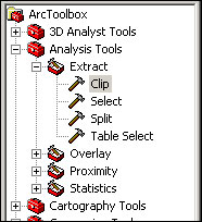
ArcToolbox is the application that provides an environment for performing geographic information system (GIS) analysis. ArcToolbox allows the user to perform a variety of geoprocessing tasks including data conversion. To access ArcToolbox, click on the ArcToolbox icon in ArcMap.
![]()
To clip one layer based on another, the user must use Clip found in the Extract portion of Analysis Tools in ArcToolbox.
Now, for completing your exercise, you will have to clip all the four layers: parcel, bldg, snd, and busstop, for the study area that you have chosen (or Capitol Hill, either way).
In the Clip dialogue box, you choose, each time, one of the four layers as the Input Features, and choose the district boundary layer as the Clip Features, and name your output layer (output feature class), or just use default name, then you click OK to finish clipping. You will see that the output layer will be added into your map.
PART G. CREATING MAPs
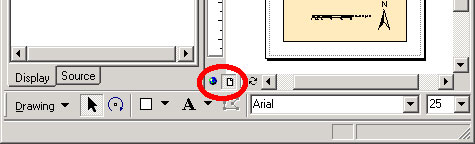
When you open ArcMap, you often view the data layer in Data View. To view the data in layout view, which is the view in which a map will be printed, the user must click on the View menu and select Layout View. Or Click on the small Layout View icon under your map content window.
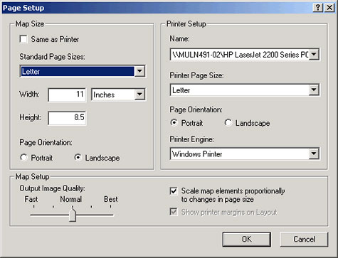
Map elements may be arranged within a variety of paper sizes. In addition, the orientation of a page may be either horizontal or vertical. It is recommended that the user specifies these characteristics before they begin the map layout process.
Paper sizes and orientation can be selected by clicking on the File menu and selecting Page Setup. The Page Setup dialog box will appear. For this exercise, use Letter size.
A map title may be added to the layout by clicking the Insert menu and selecting the Title option. A text box will be added to the page. Within this text box, a default title will be present. The user can type in a preferred title within the text box and press Enter. After the Enter key has been pressed, the user can go back and edit the title by double-clicking the on the title and editing its text properties.
The font, size, style, or color of the title may be changed using the Draw Toolbar.
A North Arrow may be added by clicking the Insert menu and selecting the North Arrow option. The user can resize the north arrow by clicking and dragging on one of its corners. In addition, the user can move the north arrow to any desired location within the map layout.
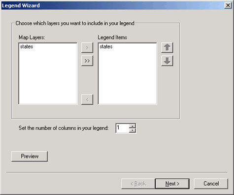
Other elements may be added include: A Scale Bar, texts, and A Legend. A Legend may be added by clicking the Insert menu and selecting the Legend option.
By default, the legend includes all layers from the map, and the number of legend columns is set to one. The user can choose which layers may be displayed in the legend by selecting the layer from the Map Layer box and clicking the right arrow (>>). The selected layers will be displayed in the Legend Items box.
PART H. SAVING YOUR DATA
The last step in this process is to save your work. While the data itself is already saved as shapefiles, you can also save your layout and symbology as an ArcMap Project File (*.mxd).
- Click on the Save button:

- You will be promted to save your file in a location in the full Windows file system. Find your working directory and save it there as something like "Exercise1.mxd".
- When you've finished this, you should exit ArcMap and ArcCatalog, then backup your ArcMap Project on your flash drive. You don't really need to backup the Shapefiles, since they are tool large to fit them all on a Zip disk, and you can always download them again from WAGDA. If you do this, however, you'll need to be sure to put the ArcMap Project file in the same place relative to the data files, so that it can easily find them in the directory system.
Last modified: 4/29/2009 12:17 PM