Prepared by Tim Brown and Cole Younger To calculate production for our scenario we used a combination of three regression equations found in a paper called, "Compendium of Cable Yarding Production Equations," by Richard R. Aubuchon. From his compilation we chose equations based on scenarios we felt matched our setting best. The paper organizes equations according to the cable system's maximum mainline pull and the type of harvest (e.g., clear-cut, partial). The type of cable system, such as running skyline, also helps categorize equations. From the Logger PC analysis we obtained the general characteristics of our setting. Table-1-- Average values for slope yarding distance (ft.), slope (%), lateral yarding distance (ft.), number of logs per turn, board-feet volume per turn, and weight per turn (lbs.) for each landing and overall harvest setting.
The numbers in Table-1 were based on Logger PC information. For instance, if Logger PC told us that Landing #2, Road # 6, had a span or external yarding distance of 1,000 feet we estimated the actual average slope yarding distance (SYDIST) to be about 750 feet. Slope was estimated from a map of slopes for the area created in GRID. Lateral yarding distance was based on the spoke dimensions defined in Logger PC. In Logger PC the analysis was based on 3.5 logs per turn for each phase of the analysis. Board-feet volume and weight per turn were estimated similarly to the method that slope distance was. We assumed utilizing a live skyline system, with a 7/8-inch mainline dimension. This cable has a maximum safe working load of approximately 27,000 lbs. (Logger PC). For our setting we were told to consider both clear-cut and selective cut. The compendium defines systems used in clear-cuts and partial cuts. We were then directed to treat a selective cut as a clear-cut for compendium purposes because it was felt the partial cut was closer to a thinning than an actual selective cut.
With these values we could select equations from the compendium based on the conditions each equation was derived under. We felt the following three equations closely matched our scenario. We made the gross assumption that the maximum safe working load is equivalent to the maximum mainline pulling load defined in the compendium. Note that according to the compendium we were using a "medium" size yarder with a maximum mainline pull greater than 25,000 pounds and less than 71,000 pounds:
The following is a little background about the conditions under which each equation was derived.
Equation II--11; (Gardner 1980) LN (TT) = 1.910023 + 0.000545 * (SYDIST) - 0.006795 * (SLOPE) + 0.002118 * (LDIST) - 0.4162 * (LOGS)^(-1) LN (TT) = Natural Log of the Turn Time in Minutes SYDIST = Slope Yarding Distance in Feet SLOPE = The Slope Measured from the Landing to the Hook Point in Percent. Percentage given as a Whole Number. For Uphill Yarding, the Value is Negative. For Downhill Yarding the Value is negative. LDIST = The Lateral Yarding Distance in Feet. This is the Actual Slope Distance the Log Travels from Hook Point to Corridor. LOGS = The Number of Pieces Yarded per Turn. In the compendium there is only one equation defined for a "medium" yarder in a live skyline system and a clear-cut situation. It is derived from a study done by Gardner in 1980. It is important to note the result is based on delay free time. The author identifies the delay percentage to be approximately 10.8 percent for this study. The system used a Link Belt HC-78B yarder and about 43-foot tower. The material removed was green and recent dead logs to 5.5-inch tops. The yarder was used in a clear-cut scenario. In this case the mainline was 1/2 inch and the tower height was about 42 feet. The system was live gravity outhaul with uphill yarding. A crew total of 5 were used and they were a commercial logging crew. The study had similar attributes in terms of slope yarding distance, lateral yarding distance and ground slope. For more in-depth information please see Compendium pages 81-103.
Equation II-10; (Gardner 1980) LN (TT) = 1.812551 + 0.000940 * (SYDIST) - 0.00950 * (SLOPE) + 0.001721 * (LDIST) + (0.00001) * (0.277323) * (LOGS) * (WEIGHT)
LN (TT) = Natural Log of the Turn Time in MinutesSYDIST = Slope Yarding Distance in Feet SLOPE = The Slope Measured from the Landing to the Hook Point in Percent. Percentage given as a Whole Number. For Uphill Yarding, the Value is Negative. For Downhill Yarding the Value is Negative. LDIST = The Lateral Yarding Distance in Feet. This is the Actual Slope Distance the Log Travels from Hook Point to Corridor. LOGS = The Number of Pieces Yarded per Turn. WEIGHT = The Turn Weight in Pounds This is the same system as above but used in a "partial cut" situation this time. Even though this system was used in a "partial" cut or thinning system we felt it was still more representative of our situation that some of the others. The result is again based on delay free time with a delay percentage of 27.8 percent. The material removed was green and recent dead logs to5.5" top. The system has the same dimensions as the above scenario so we do not list or describe them again here.
Equation III-1; (Dykstra 1) TT (min) = 4.67769 + 0.00051987 * (BFVOL) + 0.00146182 * (SYDIST) BFVOL = The Gross Board Feet Volume in the Turn, Includes Unmerchantable Pieces.SYDIST = Slope Yarding Distance in Feet The equation set forth by Dykstra incorporates a clear-cut scenario with a "large yarder" (as defined by the paper), with a maximum mainline pull of >= 71,000 pounds. The system used a Skagit BU-90 yarder and a Skagit T-90 tower. The equation is based on delay free time with a percentage delay of 9.2 %. The percent delay excludes yarding road changes (see page 106 for calculations). The system uses a Skagit T-90 tower with a skyline of 1450 ft utilizing a 1.25 inch skyline, while the system has a mainline of 1250 ft utilizing a line size of 1inch mainline. The system uses a live skyline shotgun system with an uphill single span, chokers and no swinging boom, based on a 6 person commercial logging crew. The system had long span capabilities and could handle steeper ground than our current project (see page 124 of the Compendium). The gross volume per turn (BF) was 760, and the average number of pieces per turn was 2.1. We chose this larger yarder because we were familiar with its characteristics and felt it fit, to a degree, the characteristics of our stand even though it was oversized and overpowered.
Merging of Equations In calculating production it is often difficult to find an equation where the characteristics of a study closely match your own. Consequently, you must rely on values derived for another set of inputs. In our case this was true. To alleviate this we have attempted to synthesize our own regression equation based on three defined above. The new equation will take into account all the variables of each equation and should be a very good tool to analyze production because each individual equation fit our scenario somewhat. To do this type of analysis we used EXCEL as an analysis tool because it has a convenient random number generator. Essentially what you need to do is to generate a sample of values from each equation then run regression analysis on those values. To do this, we took the three equations and coded them into EXCEL and generated production values from each using the random number generator to create values for each variable within an acceptable range of values (see Table-2). The range for these values was determined from each study. Table-2-- Acceptable range of values put into random number generator function in EXCEL. Values are based on values taken from compendium describing conditions of study.
Input of these values to a random number generator, generated the following output (see Tables-3 through Table-5). Table-3-- Values for production (i.e., turn time) based on random number generation for each variable in equation. These values are for the Gardner 11 equation (1980).
Table-4 -- Values for production (i.e., turn time) based on random number generation for each variable in equation. These values are for the Gardner 10 equation (1980).
Table-5-- Values for production (i.e., turn time) based on random number generation for each variable in equation. These values are for the Dykstra 1 equation (1975).
The objective of this analysis is to generate values that in turn can have regression analysis run on them that will result in a linear equation relating all the variables. This is necessary because each equation does not take into account the same variables as another equation. After we ran regression analysis on these values we obtained the following coefficients (see Table-6). Table-6-- Derived coefficients for "merged" equation taking into account all variables of all integrated equations. Coefficient is listed underneath the variable it is a coefficient to in "merged" equation.
With this type of analysis it is beneficial to generate as many values prior to the regression analysis as possible. As you can see we only generated about 25 values per equation. This limits the effectiveness of this analysis somewhat, but our results are still usable and practical. Based on the above information we now have the following equation: TT (min.) = 0.003234(SYDIST) + 0.021212(SLOPE) + 0.018860(LDIST) + 0.206100(LOGS) + 0.000190(BFVOL) + 0.000241(WEIGHT) This equation integrates all the variables of the 3 studies and should be a reasonable indicator of production on our setting. Base on this equation and the landing and overall setting characteristics described earlier we can arrive at production times for each (see Table-7) Table-7-- Production times for each landing and the overall setting based on values defined earlier and the regression analysis done above.
When this was done a second time to test the results of the previous analysis the following results were obtained (see Table-8). Table-8-- Values for second regression analysis done on different random values then above. Notice the turn times are similar in both cases.
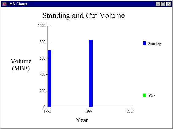
Since both methods returned similar values we have confidence that our turn time is somewhere in the range of 7.5 minutes to 7.8 minutes (delay free time). Now that we have an estimate of the turn time we can include an estimate of delay time percentage. As discussed earlier, each of the production values is based on "delay free time." Based on the values the authors gave us (e.g., 10-30%) a good estimator of percent delay would be about 20%. Therefore, any production time we calculate should have 20% added to it to compensate for delays. Based on the Logger PC analysis we know for our three landings the following information about total harvestable volume (see Figure-1 and Figure-2).
Figure-1-- Total harvestable volume in MBF in stand #23145 which contains Landing #s 2 & 5
Figure-2-- Total harvestable volume in MBF in stand #5036 which contains Landing # 3.Based on this information we have approximately 3,550 MBF of harvestable timber. Assuming all harvestable timber was removed by cable yarding--which it is not, some is harvested by shovel--then the following can be concluded. I assume that a truckload of logs is typically around 5,000 MBF and that a turn typically has about 850 board-feet volume. Therefore, if it takes 7.5 minutes (based on values in Table-7) per turn plus 20% delay time then each turn takes approximately 9 minutes. In an 8-hour day (working continuously) you could get about 53-54 turns in or about 45,500 board feet per day. Assuming a truckload is equivalent to 5,000 MBF that is about 9-10 truckloads per day. At this rate, it would take approximately 75-80 days to log this whole setting assuming it was all done under the conditions describe above. Back to outline
|


