Orthophotos exist for the entire state of Washington. They can be obtained as a "tif" image which consists of pixels or cells of size 3 by 3 ft, each with a grayscale ranging from 0 to 255. Use of these 256 shades of data were investigated for usefulness in extending the LULC (land use land cover) and HYDRO (hydrology) layers. Two simple pieces of information were sought within the scope of this class: (1) trees vs no - trees indicating forest; and (2) presence or absence of an opening or gap indicating presence of a stream. The major drawback to using data (grayscales) from a photographic image (orthophoto) is misinformation due to shadows. For example, a clear cut with no trees on the shaded side of a slope may exhibit the same grayscale as a dense forest positioned on the sunny side of a slope. Intuitively, therefore, no clear direct correlation on a cell by cell basis can provide reliable results.

The current simple approach for both trees and a stream gap is to select training sets of pixels where we know trees or a stream gap occurs. Then use the range of cells that occur most often in a histogram of the cell values from the training set for a display from the orthophoto. If those cells displayed correspond to known tree or stream gap areas, then this simple approach could be used.

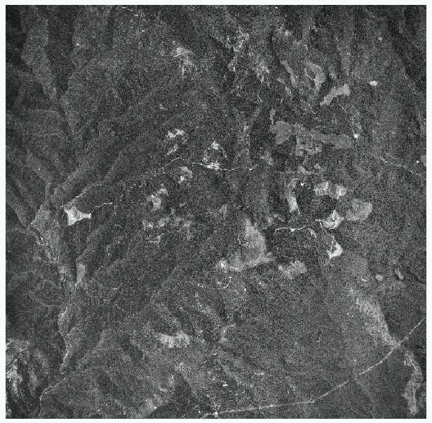
 Figure 1. Entire ortho area used for this study which was 1 of 4 covering the entire Washougal area . (entire_ortho.gif)

The application of orthophoto grayscales for use in extending the LULC (land use land cover) layers was investigated in this section. The approach was to see if gap vs no gap or trees vs no - trees could be determined from the orthophoto. To accomplish this, training areas were chosen in two different looking areas each in clearcut and timbered areas. Histograms were then formed from each pair of training areas and the range of grayscales were displayed (see figures 4 and 8). The range of most frequently occurring grayscale values was chosen to form a grid coverage identifying those pixels that matched the range as black and those that were outside the range as bright green. Comparative views are then presented that show the orthophoto area beside the grid (see figures 2, 3, 5, 6, 9, and 10). These are visual examples of how well the range chosen was able to identify clearcut or timbered areas. For example, if you view several patches of clearcuts on the orthophoto, but their shapes are indistinguishable on the grid, then this simple approach was unable to differentiate clearcut areas.

Clearcut differentiation

Timber area differentiation

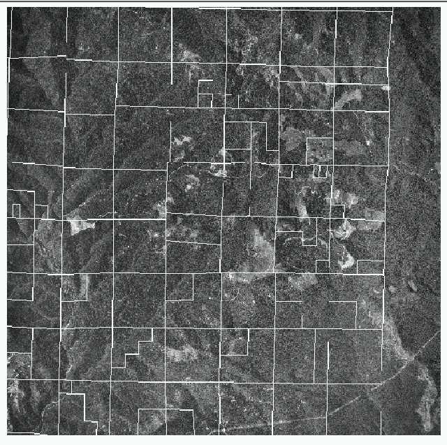
Utilization of grayscales to determine timber areas was more promising than for the clearcuts. The histogram (figure 8) based on the training pair (figure 7) shows the range of most frequently occurring grayscale values (31 to 75) is slightly more narrow than that used for clearcut (60 to 115) and covers almost entirely a different range. Examination of the entire orthophoto and the grid formed using the range of 31 to 75 (figures 9 and 10) show the grid identifies timbered areas in a pattern very similar to the orthophoto itself.

These results prompted extraction of actual data for more rigorous statistical testing. Since visually there appeared to be a high correlation, it was possible there would be some direct correlation between orthophoto grayscale and some LULC polygon value such as BA/acre (basal area per acre). All the LULC layer data that occurred in the orthophoto area were extracted and joined with a grid formed from the orthophoto layer. The grid value from the orthophoto layer was the average grayscale that occurred in a LULC polygon. All this data was then summarized and exported as a comma delimited ascii file. This file was examined in MS Excel and cells with zero values were eliminated. The remaining rows were exported as a comma delimited text file and used as input for regression analysis in SPSS (Statistical Package for the Social Sciences).

Although the orthophoto and grid layer indicated promising results visually, the actual data associated with the pixels showed poor correlation (see Table 1). The over-riding reason for this is likely due to the fact that we are not comparing pixel to pixel but the average of an entire LULC polygon that may range from a few acres to hundreds of acres. For example, if each polygon was stratified into subunits that exhibited similar grayshade scales and then the actual ba/acre, etcetera could be known for the subunit the correlation would likely have been stronger. Still, of course, angle of the sun and side of the slope the timber is on may cause shadows that mask any true relationships. If the visual results are real, other class groups could fill in missing LULC layers by using grayscale shades between 31 and 75 to indicate presence of timber. Taking various transformations of the variables, such as square, logs, and inverse did not help singificantly in improved correlations.

Table 1. Results of stepwise regression betweeen orthophoto average grayscale per LULC polygon and LULC polygon values.

(Note: ba/acre = basal area per acre; dbh/acre = diameter at breast height per acre; stems/acre = number of stems per acre less than 7 inches dbh; average grayscale was the average of all grayscale values found in each polygon)

The dark pixels displayed in the grid formed (figure 14) indicate all pixels with a range of 85-130 grayscale shade value. The green area is all pixels outside of that range. The hydro stream layer is also superimposed to indicate where known streams occur. The orthophoto (figure 13) shows approximately the area represented by the grid. Note how many "stream gaps" are indicated where known hydro vectors don't occur.

 The orthophoto and grid covering the entire area (figure 15 and 16) depict the same 85-130 grayscale shade range. There is no hydro layer superimposed because it would obscure details at this scale. Note how the clearcuts and many hill sides are displayed as "stream gaps".

The range of grayscales chosen for a clearly define gap appears to be too wide to prevent calling many other non-gap items as gaps. An improvement on this method would be to use distance from a known hydro layer stream vector in choosing which pixels to use for gap analysis. But given the high degree of shading as stream size becomes smaller, it us unlikely that orthophoto grayscales alone can give reliable results.

Currently the following ground and photographic/map methods are used to collect LWD, canopy closure, and channel info as given in the 1995 version of the Watershed Analysis manual.

(a) LWD - aerial photographs & ground truthing.

(b) Canopy closure - aerial photos & ground truth with densiometer.

There are various alternative approaches to enhancing existing LULC and riparian buffer layer information with various forms of existing imagery beyond using the digital black and white orthophotos directly. For example:

The weakness with any approach is to try and develop relationships from spectral images from satellites or orthophotos without using ground truthing and existing or new aerial photography. We strongly urge that those two aspects not be ignored in the development of any relationships that are intended for actual management use. The following provides more details about these three alternative approaches.

A step by step approach for a class project to enhance stream information of LWD, canopy closure, and channel information:

1. Obtain 1, 2, or 3 pairs of stereo aerial photos as diapositives (1:12,000 or 1:15840) that cover streams in the Washougal area and were used for the digital ortho photo coverage.

2. Using the AP190 analytical plotter, transfer ground control to the stereo aerial photos.

3. Digitize watercourses on the stereo aerial photos.

4. Evaluate canopy closure within 66 ft buffers along the water courses.

5. Determine LWD recruitment potential based on Watershed Analysis methods from aerial photo examination by using high, medium, and low values based on dominant tree type and age/size class and density.

6. Determine channel width estimates where visible from aerial photos.

7. Convert aerial photo evaluation to a 3 x 3 ft grid.

8. Convert 30 x 30 m HYDRO layer to a 3 x 3 ft grid.

9. Convert 30 x 30 m LULC layer to a 3 x 3 ft grid.

10. Export as ascii data, the coordinates and gray scale from ORTHO layer.

11. Export as ascii data, the coordinates and water course and water boundary values from HYDRO layer.

12. Export as ascii data, the coordinates and stand information from the LULC layer (eg average dbh, ba/acre, stems/acre < 7", bdft/acre, etc)

13. In a statistical package, perhaps using regression analysis, try to predict the cell values for canopy closure, LWD, and channel width determined from the aerial photo interpretation by using the ORTHO, LULC, and HYDRO cell values as independent variables. Or alternatively join all of these attributes in Arc/Info before exporting.

14. If a reasonable correlation emerges then we could apply the equation to determine canopy closure, LWD, and/or channel width values or categories for the watershed area.

 To enhance layers of timber, the same process of mounting the aerial photos on the AP190 transfer of ground could be followed. Then smaller polygons of timber types could be digitized that would be within existing polygons from the LULC layer that overlay the orthophoto. Since locations of these points would be known, field visits could be made and stand data collected that would provide a higher resolution of stand information. With this better information training areas on the orthophotos could be examined and relationships developed. If some ground truthed areas are kept aside, these could be used for testing the accuracy of the developed relationships.

Obtain satellite and orthophoto imagery from over the same watershed area. Use Imagine (software) to join the spectral bands from both sets of imagery. Pursue relationships between these spectral bands and existing LULC and hydro layers. Ideally this should be linked as in current methods with aerial photos and ground truthing. Several sample areas on the ground of known locations that correspond to the imagery locations should be visited and assess the variables of interest and note their representation on the aerial photography. Then using this information develop training areas for the spectral bands and develop relationships, through regression analysis for example.

This approach would make use of new technology. The idea is that with higher resolution digital orthophotos, detailed images similar to aerial photos would be available which contain more information that could be used for LULC and hydro layer enhancement. The aerial photo diapositives are scanned and then loaded into an analytical plotters computer for automated digital orthophoto production. These new digital photos would require larger amounts of disk space but provide more detailed images.

BACKGROUND Orthophotos are 4 or 5 generations removed from the original aerial photography. The resulting information to be obtained is greatly decreased because of the lower resolution. Normally orthophotos are in greatest demand for use as base maps. With an orthophoto, the forester, range manager, engineer, or geologist can correlate images on the photo with those observed in the field much more easily than with a conventional line map. Knowing the scale of the orthophoto, the land manager can make direct measurements on the orthophoto with accuracy. Field observations can also be plotted accurately on orthophotography without first making a base map.

ORTHOPHOTOGRAPHY - An orthophoto is a photo reproduction that has been corrected for tilt, topographic displacement, and sometimes camera lens distortion. Orthophotos are produced from sterescopic pairs or triplicates of aerial photographs by a process called differential rectification so that the resulting photographic images are in a correct orthographic position.

The production of an orthophoto entails the conversion of conventional photography by utilizing a double-projection orthophotoscope. The anaglyph principle: Most orthophotos are produced through the use of diapositives and direct optical projection systems that use the anaglyph principle. An anaglyph consists of the two superimposed images of the overlapped portion of a stereoscopic pair of photos. These superimposed images are produced by double-projection optical systems within most orthophotoscopes by placing red and blue filters between the light source and the diapositives -- a different colored filter for each projector. The three-dimensional model, as viewed through colored glasses (also red and blue), is projected by the orthophotoscope onto a film carrier than can be raised and lowered by the operator. The table carries a photographic film (the film plane) that is sensitive only to blue light. When exposed and developed, this film becomes the orthophoto negative.

The quality of orthophotography is generally lower than that of standard photography. There are problems of tone matching between scanning strips, visible scanlines, image blurring, duplication of imagery, gaps, and scanline discontinuities. The most troublesome problems are created when scanning steep terrain. Blurring can occur due to rapid up and down movement of the filme plane. Electronic scanning helps eliminate this. Resolution of the final imagery is less than the original photograph, primarily because the final image is frequently four to five generations removed from the original.

New methods exist, but this at least gives some principles.

(source: Paine, D. P., Aerial photography and image interpretation for resource management. 1981, John Wiley & Sons, Inc.)