Model Fitting
In this lesson we'll cover how to fit a model to data using matlab's minimization routine 'fminsearch'. Model fitting is a procedure that takes three steps:
First you need a function that takes in a set of parameters and returns a predicted data set.
Second you need an 'error function' that provides a number representing the difference between your data and the model's prediction for any given set of model parameters. This is usually either the sums of squared error (SSE) or maximum likelihood.
Third you need to find the parameters that minimize this difference. Once you set things up properly, this third step is easy thanks to the nerds at Mathworks.
Contents
- One parameter example - Weber's law
- Step 1: model prediction
- Step 2: Comparing the model prediction to the data
- Step 3: Finding the best fitting parameter
- Other measures of error
- Model fitting weighting by standard error of the mean.
- Model fitting weighting by individual measurements.
- Model fitting with more than one parameter.
- Holding variables constant while fitting.
- Other notes.
One parameter example - Weber's law
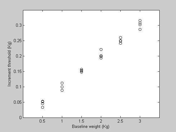
We'll start with a simple example where our model has just one parameter. Weber's law states that the ability for a subject to notice an increase in stimulus intensity is proportional to the starting, or baseline intensity. That is, if x is the stimulus intensity, the increment threshold is kx, where k is the 'Weber fraction'. This fraction is our one parameter.
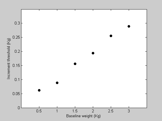
Suppose that we ran an experiment testing the ability for a subject to detect an increase in the weight of an object held in the hand. Subjects were given starting weights (in Kg) of the following values:
clear all
x = [.5,1,1.5,2,2.5,3];
Increment thresholds are defined here as the increase in weight that can be detected correctly 80% of the time. This would use a psychophysical method such as 'two-alternative forced-choice' (2AFC) that we don't need to deal with right here. Let the corresponding increment thresholds for a subject be:
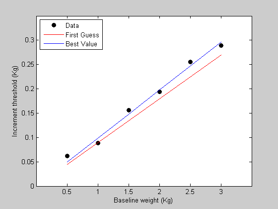
y = [  0.0619    0.0888    0.1564    0.1940    0.2555    0.2890];
%Let's plot the data:

figure(1)
clf
h1=plot(x,y,'ko','MarkerFaceColor','k');
set(gca,'YLim',[0,0.35]);
set(gca,'XLim',[0,3.5]);
set(gca,'XTick',x)
xlabel('Baseline weight (Kg)');
ylabel('Increment threshold (Kg)');
Step 1: model prediction
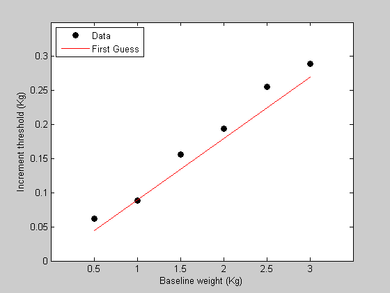
We're now ready for the first step - writing the function containing the model that predicts the data. This function needs to take in a single parameter and the baseline weights and return a prediction of the data. The parameter is the WeberFraction which is the slope of the line of the data in figure 1.
We'll use a specific convention for how we represent our parameters which is to place them inside a single structure. With one parameter this seems a little silly, but it'll make sense when we add more parameters.
Here's a structure containing a starting guess at the Weber fraction 'w':
startingW  =0.09;  %make this a variable to use later.
p.w = startingW;
Our function 'predictWeight' is a single line function that will take in this structure as its first argument, and the list of baseline values as the second argument:
%%%%%%%%%%%%%%%%%%%%%%%%%%%%%%%%%%%%%%%%%%%%%%
%function pred = WebersLaw(p,x)
%
%pred = p.w*x;
%
%%%%%%%%%%%%%%%%%%%%%%%%%%%%%%%%%%%%%%%%%%%%%%

pred = WebersLaw(p,x);
plot the prediction
hold on
h2=plot(x,pred,'r-');
legend([h1,h2],{'Data','First Guess'},'Location','NorthWest');
Step 2: Comparing the model prediction to the data
Time for step 2. Here's a two-line function 'WebersLawErr' that calculates the sums of squared error between the model's prediction and the data:
%%%%%%%%%%%%%%%%%%%%%%%%%%%%%%%%%%%%%%%%%%%%%%
% function err= WebersLawErr(p,x,y)
%
% pred = WebersLaw(p,x); err = sum( (pred(:)-y(:)).^2);
%%%%%%%%%%%%%%%%%%%%%%%%%%%%%%%%%%%%%%%%%%%%%%
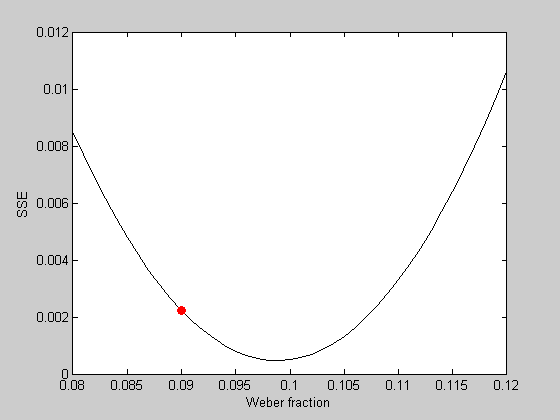
%The SSE between our model and the data for our first guess is:

err = WebersLawErr(p,x,y)
err =

    0.0022
Step 3: Finding the best fitting parameter
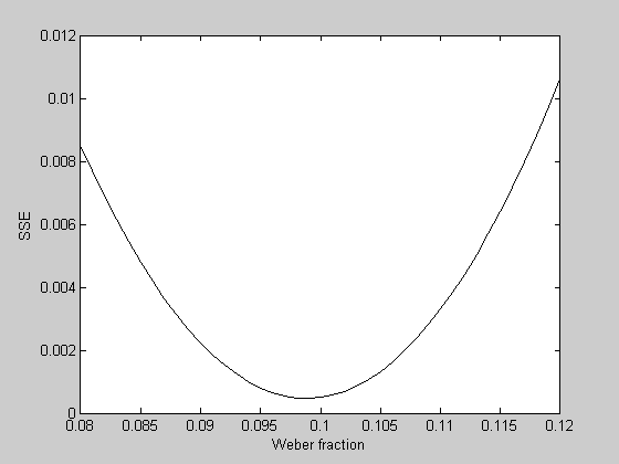
What is the best fitting Weber fraction? With one parameter we can visualize this problem by calculating the error of the fits for a range of Weber fractions:
WeberList = linspace(0.08,0.12,41);
errList = zeros(size(WeberList));
for i=1:length(WeberList)
    p.w = WeberList(i);
    errList(i) = WebersLawErr(p,x,y);
end

figure(2)
clf
plot(WeberList,errList,'k-');
xLabel('Weber fraction');
yLabel('SSE');
We can plot the error value of our initial guess in red:
hold on
plot(startingW,err,'ro','MarkerFaceColor','r');
It looks like the best fitting Weber fraction is between 0.095 and 0.1. We could go further and keep sampling finer and finer in this range to find a minimum value. But this is a very inefficient way to find the minimum of a function. It's especially bad if there are multiple parameters to fiddle with.
Fortunately, matlab has a function 'fminsearch' that uses a sophisticated numerical analysis technique that can find the minimum of a function like this - as long as it's reasonably continuous and well behaved. I find Matlab's usage of fminsearch to be a bit kludgy and awkward, so I've written my own function that calls 'fminsearch' that I find easier to use. It's called 'fit.m', and it works like this:
help fit
 [params,err] = fit(funName,params,freeList,var1,var2,var3,...)

 Helpful interface to matlab's 'fminsearch' function.

 INPUTS
  'funName':  function to be optimized.  Must have form err = <funName>(params,var1,var2,...)
  params   :  structure of parameter values for fitted function
      params.options :  options for fminsearch program (see OPTIMSET)
  freeList :  Cell array containing list of parameter names (strings) to be free in fi
  var<n>   :  extra variables to be sent into fitted function

 OUTPUTS
  params   :  structure for best fitting parameters
  err      :  error value at minimum

 See 'FitDemo.m' for an example.

 Written by Geoffrey M. Boynton, Summer of '00

    Overloaded methods:
       gmdistribution/fit
The first argument that 'fit' needs is the name of the function to be minimized, as a string. In our case it's 'WeberListErr'. This function has to have the convention that it's first argument is a structure containing the model parameters, and that the first argument it returns is the error value. The function can take in additional arguments too, in any order.
The second argument into 'fit' is a structure containing a starting set of parameters. This is the first guess for where the minimum is, and it can make a difference in the ability for fminsearch to find the overall minimum.
The third argument is a cell array containing a list of parameters that we will allow to vary to find the minimum. The cell array is a list of strings containing fields of the names of the parameters in our structure. In our case, it's just a single field named 'w'.
The remaining arguments into fit are the remaining arguments that the function to be minimized needs, starting with the second argument. In our case they are the parameters x and y, in proper order.
The first argument in the output of 'fit' is a structure containing the best-fitting parameters. The second argument is the error associated with these values.
Let's go!
[bestP,bestErr] = fit('WebersLawErr',p,{'w'},x,y);
Fitting "WebersLawErr" with 1 free parameters.
'bestP' is a structure containing the parameters that minimized the SSE between the data and the model.
bestP
bestP =

    w: 0.0988
We can plot this in figure 2
hold on
plot(bestP.w,bestErr,'bo','MarkerFaceColor','b');
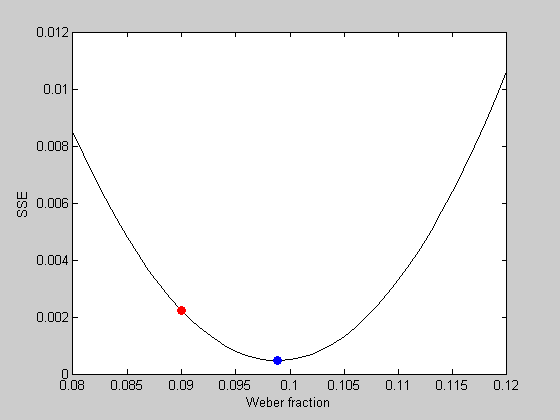
See how it sits on the bottom of the curve? We found the optimal Weber fraction that fits our data. About 0.1033 (or 10.3%)
Finally, we'll get the model prediction using this best fitting value and plot the predictions with the data in figure 1
bestPred = WebersLaw(bestP,x);
figure(1)
h3=plot(x,bestPred,'b-');
legend([h1,h2,h3],{'Data','First Guess','Best Value'},'Location','NorthWest');
Other measures of error
The best fitting parameters can depend strongly on your choice of error function. For our example, another way to state Weber's law is that the ratio of the increment thresholds and the baseline values is constant. So another measure of the Weber fraction is the mean of these ratios across baselines:
meanRatio  = mean(y./x)

% This gives a slightly different answer:

disp(sprintf('Best w: %5.4f, mean ratio: %5.4f',bestP.w,meanRatio));
meanRatio =

    0.1021

Best w: 0.0988, mean ratio: 0.1021
This difference is at least in part caused by a greater weight for the mean ratio on the lower baseline values (or equivalently a greater weight for the high baseline values for the model). It's not obvious which is more valid. The model puts equal weight on absolute errors in the 'y' dimension across baselines, while the mean ratio puts equal weights on the ratios across baselines.
Model fitting weighting by standard error of the mean.
The mean ratios might be a better method because thevariability in the data (which we haven't yet talked about) probably increases with the baseline. So errors at high baselines are less meaningful than at low baselines.
A natural way to correct for variance in the data is to normalize the SSE by the standard error of the mean for each data point. Then our error value will represent a total error in sqsuared standard error units.
Let the standard error of the mean of our estimates be:
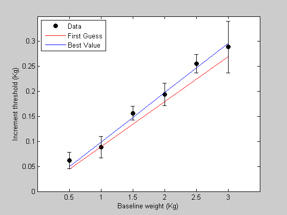
s =  [ 0.016    0.0216    0.0140    0.0225    0.0183    0.0517];

% Plot these error bars in figure 1:

figure(1)
h=errorbar(x,y,s,'k','LineStyle','none');
Next, edit the 'WebersLawErr' function to this:
%%%%%%%%%%%%%%%%%%%%%%%%%%%%%%%%%%%%%%%%%%%%%%
% function err= WebersLawErr(p,x,y,s)
%
% if ~exist('s','var')
%     s = ones(size(x));
% end
%
% pred = WebersLaw(p,x); err = sum( (pred(:)-y(:)).^2./s(:).^2);
%%%%%%%%%%%%%%%%%%%%%%%%%%%%%%%%%%%%%%%%%%%%%%
%
% And use this new error function to find the best fitting parameters:

[bestPsem] = fit('WebersLawErr',p,{'w'},x,y,s);
%
% Get the new model predictions and plot it in figure 1
%
bestPredsem = WebersLaw(bestPsem,x);
figure(1)
h4 = plot(x,bestPredsem,'k-');
legend([h1,h2,h3,h4],{'Data','First Guess','Best fit using SSE','Best fit using standard errors'},'Location','NorthWest');
Fitting "WebersLawErr" with 1 free parameters.
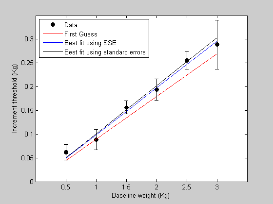
The new best fit takes into account the error bars so that data points with smaller error bars are weighted more heavily. You can think of this as making the model prediction overlap more with the error bars, rather than simply trying to get close to the data points.
In this example, the last data point (highest baseline value) is noisy, so the model's constraint to fit this point is relaxed. This causes the best fitting Weber fraction to change so that the prediction moves away from this noisy data point.
Model fitting weighting by individual measurements.
Another way to account for the variability in your measurements is to use an error function that sums up the errors with respect to each individual measurements, rather than the means. This is closely related to the previous method - it's identical in the limit as you add more and more measurements to each mean.
We'll start with a new sample data set from the Weber's law experiment that has four measurements for each baseline intensity. We'll call the variable 'yy' instead of 'y'.
yy=[0.0457    0.0885    0.1533    0.1941    0.2607    0.3029;
    0.0333    0.1119    0.1517    0.2218    0.2506    0.2866 ;
    0.0513    0.1119    0.1481    0.1986    0.2490    0.3071 ;
    0.0529    0.0996    0.1573    0.2011    0.2417    0.3162];
Each of the 4 rows corresponds to a separate measurement across the 6 baseline values.
An easy way to compare these values to the model's prediction is to make the model predict a data set that's the same size as yy. This can be done by using a matrix xx that's the same size too:
xx = repmat(x,4,1)
xx =

    0.5000    1.0000    1.5000    2.0000    2.5000    3.0000
    0.5000    1.0000    1.5000    2.0000    2.5000    3.0000
    0.5000    1.0000    1.5000    2.0000    2.5000    3.0000
    0.5000    1.0000    1.5000    2.0000    2.5000    3.0000
We can plot this new data set as individual data points:
figure(3)
clf
h1=plot(xx,yy,'ko')
set(gca,'YLim',[0,0.35]);
set(gca,'XLim',[0,3.5]);
set(gca,'XTick',x)
xlabel('Baseline weight (Kg)');
ylabel('Increment threshold (Kg)');
h1 =

  528.0250
  936.0029
  937.0029
  938.0029
  939.0029
  940.0029
It turns out that we've written our model function 'WebersLaw' so that it can take in matrices as well as vectors, so it will also make a predicted data set that's a matrix:
pred = WebersLaw(p,xx)
pred =

    0.0600    0.1200    0.1800    0.2400    0.3000    0.3600
    0.0600    0.1200    0.1800    0.2400    0.3000    0.3600
    0.0600    0.1200    0.1800    0.2400    0.3000    0.3600
    0.0600    0.1200    0.1800    0.2400    0.3000    0.3600
We've also written our error function 'WebersLawErr' so that it can calculates the SSE between the elements of two matrices as well as vectors, since we unwrapped our variables using the '(:)' method:
err = WebersLawErr(p,xx,yy)
err =

    0.0346
This means that our fitting routine will work too:
bestP = fit('WebersLawErr',p,{'w'},xx,yy);
Fitting "WebersLawErr" with 1 free parameters.
To get a prediction of the model with this best-fitting value of w, we only need a single vector instead of the whole matrix. We can do this by sending in the variable 'x' instead of 'xx' in to 'WebersLaw':
pred = WebersLaw(bestP,x);
Plot it:
hold on
h2=plot(x,pred,'k-');
legend([h1(1),h2],{'Data','Best fitting model'},'Location','NorthWest');

Model fitting with more than one parameter.
Fitting a model that has more than one parameter is easy, since the hard part of actually finding the best parameters is all done by Matlab's fminsearch function. Here's an example of a data set that needs a two-parameter model to fit it.
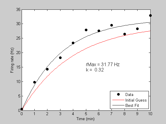
Suppose we're measuring the firing rate of a neuron while it is recovering from an adapted state. Let 't' be time in seconds, and 'y' be the firing rate of the neuron. Here's an example data set:
t = [0:10];


y=  [0.4346    9.8079   14.2634   18.2656   23.4209   27.8469   27.5358 ...
     29.4886   26.4415   28.2591   32.8832];
Plot the data
figure(5)
clf
h1=plot(t,y,'ko','MarkerFaceColor','k');
xlabel('Time (min)');
ylabel('Firing rate (Hz)');
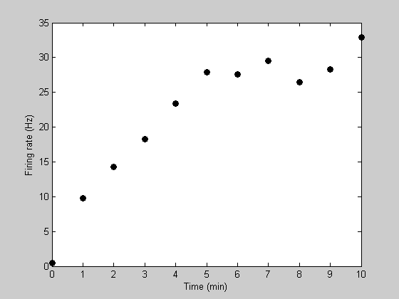
Notice how the recovery from adaptation starts out quickly and then asymptotes to a firing rate of about 30Hz. A standard model for this sort of asymptotic function is an exponential. This can be described with two parameters - one describing the asymptotic firing rate (we'll call it 'rMax') and a second one decribing the rate of recovery (we'll call it 'k').
We need to do steps 1 and 2 now from above - write the function containing the model and write a function comparing the model to the data. This time we'll do it a little differently and combine the two into a single function, called 'predRecoveryErr':
%%%%%%%%%%%%%%%%%%%%%%%%%%%%%%%%%%%%%%%%%%%%%%
%
% function [err,pred] = predRecoveryErr(p,t,y)
%
% %model goes here. pred = p.rMax*(1-exp(-p.k*t));
%
% %SSE calculation goes here. if exist('y','var')
%     if ~exist('s','var')
%        s = ones(size(y));
%     end
%
%     err = sum( (pred(:)-y(:)).^2./s.^2);
% else
%     err = NaN;
% end
%
%%%%%%%%%%%%%%%%%%%%%%%%%%%%%%%%%%%%%%%%%%%%%%
This function returns the error value as the first parameter and the model prediction as the second. The third input parameter - the data - is optional. If it isn't provided, then no comparison is made to the data and a NaN is returned for the error. This way, the same function can serve both as a way to get model predictions, and to feed into 'fit.m' to find the best fitting parameters.
Notice that the model itself is just one line again: p.rMax*(1-exp(-p.k*t))
We're ready to use this function to predict and fit data.
Intial parameters:
clear p
p.k = .25;
p.rMax = 30;
Initial model prediction. Let's get fancy and use a higher sampling rate in time for the model prediction to get a smoother curve. Instead of predicting with the variable 't', we'll use:
tPlot = linspace(0,10,101);

[tmp,pred] = predRecoveryErr(p,tPlot);

hold on
h2=plot(tPlot,pred,'r-');
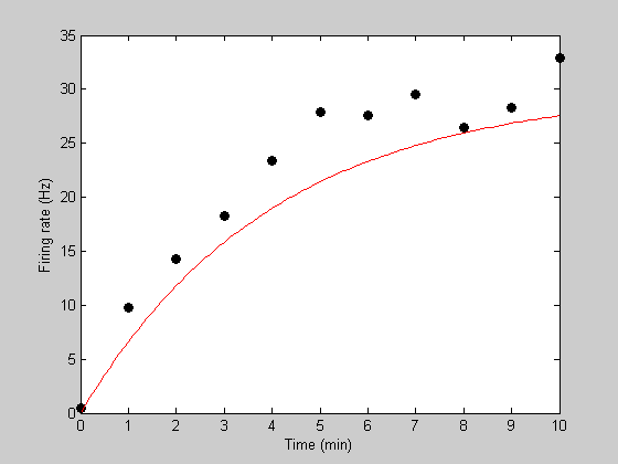
Intial error value:
err = predRecoveryErr(p,t,y)
err =

  154.4481
Find the best fitting parameters:
Our call to 'fit' will be just as in the one parameter case, except that we'll list two parameters in our cell array (3rd argument into 'fit'):
bestP = fit('predRecoveryErr',p,{'k','rMax'},t,y);
Fitting "predRecoveryErr" with 2 free parameters.
Now we'll get the best fitting prediction and plot it in black
[bestErr,bestPred] = predRecoveryErr(bestP,tPlot);

h3=plot(tPlot,bestPred,'k-');
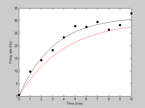
Show the parameter values on the plot:
text(5,15,sprintf('rMax = %5.2f Hz\nk = %5.2f',bestP.rMax,bestP.k),'HorizontalAlignment','left','FontSize',12);
legend([h1,h2,h3],{'Data','Initial Guess','Best Fit'},'Location','SouthEast');
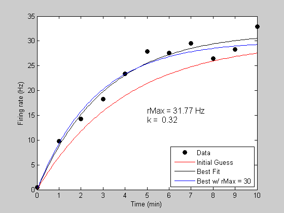
Holding variables constant while fitting.
The 'fit' function lets you easily fit with a subset of parameters. Suppose that you know that the asymptotic firing rate is 30Hz, and we just want to let the parameter 'k' vary. We do this by only listing 'k' as a free parameter in third argument to 'fit':
bestPK = fit('predRecoveryErr',p,{'k'},t,y);
[bestErrK,bestPredK] = predRecoveryErr(bestPK,tPlot);

h4 = plot(tPlot,bestPredK,'b-');
legend([h1,h2,h3,h4],{'Data','Initial Guess','Best Fit','Best w/ rMax = 30'},'Location','SouthEast');
Fitting "predRecoveryErr" with 1 free parameters.
Other notes.
'fit' allows parameters for your model to be vectors as well. For example, if you had a model with parameters:
p.x = [2,4,6];
You could allow all three values in x to be free by using {'x'} as your list of free parameters. If you want only the first element to be free, use {'x(1)'}. For just the first and 3rd, you can use {'x([1,3])'}, or {'x(1)','x(3)'}. Either will work.