SMARTPsych SPSS
Tutorial
Between-Subjects
Analysis of Variance
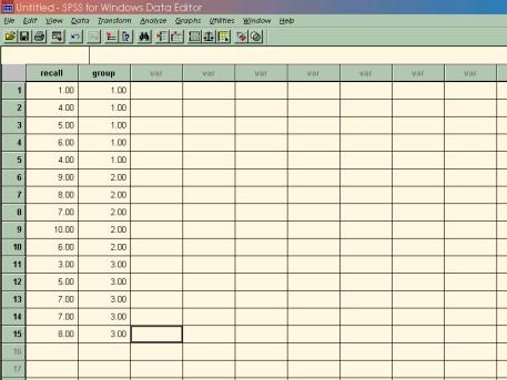
Step 1: Enter your data.
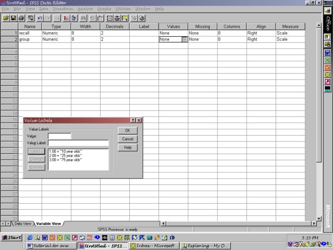
Step 2: Define your variables.
Remember that to do this, you can simply double-click at the top of the variable’s column, and the screen will change from “data view” to “variable view,” prompting you to enter properties of the variable. For your dependent variable, giving the variable a name and a label is sufficient. For your independent variable (the grouping variable), you will also want to have value labels identifying what numbers correspond with which groups. See the following figure for how to do this.
 Step
3: Select Oneway ANOVA from the command list in the menu as follows:
Step
3: Select Oneway ANOVA from the command list in the menu as follows:
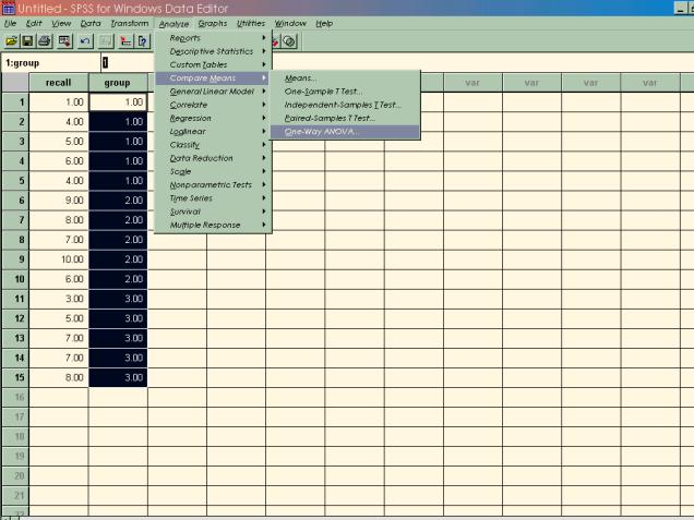
Note: There is more than one way to run this
command in SPSS. For now, the easiest
way to do it is to go through the “compare means” option. However, since the analysis of variance
procedure is based on the general linear model,
you could also use the analyze/general linear model option to run the
ANOVA. This command allows for the
analysis of much, much more sophisticated experimental designs than the one we
have here, but using it on these data would yield the same result as the
One-way ANOVA command.
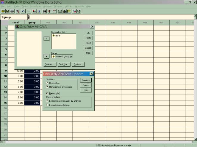
Step 4: Run your analysis in SPSS.
Once
you’ve selected the One-way ANOVA, you will get a dialog box like the one at
the top. Select your dependent and
grouping variables (notice that unlike in the independent samples t-test, you
do not need to define your groups—SPSS assumes that you will include all groups
in the analysis.
![]()
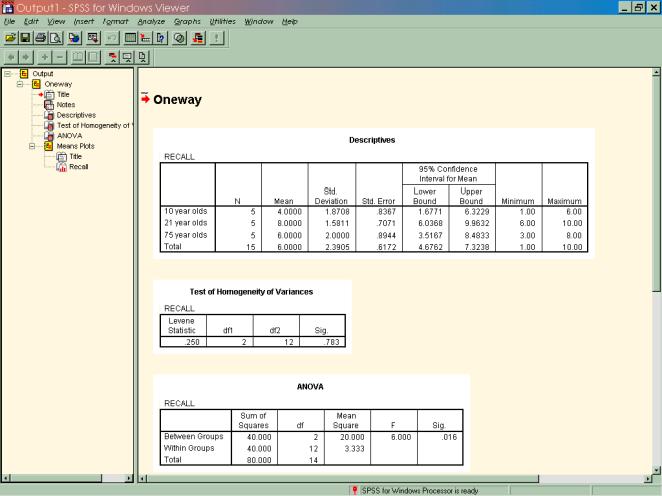
Step 5: View and interpret your output.
But
some of you are begging to know, how can I do all of this with syntax commands?
You can see what the syntax looks like by selecting “paste” when you are in the One-way ANOVA dialog box.
Step 6: Now that you know how to run a between-subjects
ANOVA, enter the data from the following problem and run through the previous
steps on your own.
In a verbal learning task, nonsense syllables are presented for later recall. Three different groups of subjects see the nonsense syllables at a 1-, 5-, or 10-second presentation rate. The data (number of errors) for the three groups are as follows:
1-second group 5-second group 10-second group
13 11 3
15 14 5
15 13 6
12 12 6
13 16 9
12 12 7
9 11 2
8 9 4
15
10 3
12 8 1
8 9 8
a.)
Do
a boxplot to see what the distributions look like.
b.)
Perform
an ANOVA on the data.