To demonstrate SPSS’s one sample t-test command, we have
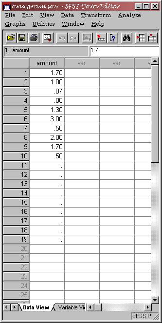
the data set to the left. These data were collected in an experiment in which
students (10 groups of 5 individuals) solved a number of complicated
anagrams in groups. One person in
each group was randomly assigned anagrams that were far more difficult than
those that the others received.
Participants were asked to allocate a $10 prize among the members of
the group in any manner that they wished.
The dependent variable is the amount of money allocated to the
“least helpful” partner in each of the groups (almost always, the person
who had the most difficult anagrams to solve). The null hypothesis is that all members of the group
would receive equal allocation of the $10 prize. Thus, the null and alternative hypotheses are: Ho: μ = 2
(they allocate the $10 equally, so each person gets $2) H1: μ ≠
2 We want to subject these data to a one sample t-test of
the null hypothesis above. Use a two-tailed test, α = .05. Click here for the
data set (you must save it to disk in order to access the file).
Once
you have the data, it is fairly simple to compute a one-sample t-test in
SPSS. Choose, from the menu,
ANALYZE / COMPARE MEANS / ONE SAMPLE T TEST
You
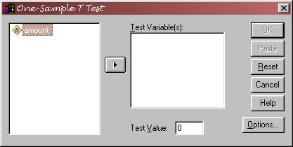
will get the dialog box that appears below:
Your
test variable is amount; click this over into
the test variable column.
What is your test value? It is the
value of the mean under the null, in this case, 2. Enter 2 into the test value box.
You
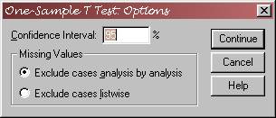
may want to check out the “options” box to see what is available to you. The box is below.
Note
that will automatically get the SPSS default 95%
confidence interval for the data.
The missing values command tells SPSS how to deal with missing data; the
SPSS default is fine for most purposes (this will become more critical when you
are dealing with more variables and have missing data in your set).
Click
OK once you have set up your dialog boxes
correctly, and SPSS will run the test.
The
output that you will receive is below:


Take
a moment to see what you have here. Of
course, your critical information is the t value
(-2.74), your degrees of freedom (9), and the significance of your test (.023;
notice that you can get exact p-values in SPSS). You also get your sample mean, the standard
deviation (this is the estimated standard
deviation), and the estimated standard error of the mean. You could compute the t-test yourself with
this information:
t = 1.177 – 2
= -2.74
.9499 / √10
Also
note that your 95% confidence interval of the difference ranges from
–1.50 to -.14. It’s strange that SPSS
computes the confidence intervals this way, but you can easily get the
confidence intervals around the mean as follows:
If
you were to compute the confidence intervals by hand, you would calculate
Mean
+/– tcrit (α=.05, 2 tailed) * σ hat / √N
Or
1.177 +/– 2.262 * .9499 / √10, the confidence interval is .4975 to 1.8565
Because you use +/- .6795 to give the bounds of your interval. Using these values around the mean difference (-.8230) you get the SPSS values; using these values around the mean (1.177) you get .4975 to 1.8565. These are the values we would use.
What would a confidence interval look like if you were using a lower alpha level (i.e., having a greater % confidence)? Let’s try using a 99% confidence interval. Run the t-test as before, but select in the options that you want a 99% c.i..

You
will get the table above. Notice that
your confidence interval is now larger (this makes intuitive sense; to have a
greater degree of confidence, you would need a larger range of possible
values). This time, the confidence
interval of the difference contains 0 (this is essentially the same as stating
that the confidence interval around the mean contains 2 (c.i. around the mean
would be .201 to 2.153).
In other words, if you use an α level of .01, you will fail to reject the null hypothesis, and your confidence interval would contain the null value. You can see that your exact p-value is .023, too high to reject the null if α is .01.
Now let’s do a paired-groups
t-test. The example for this problem
comes from the Implicit Assumptions Test (IAT). If you are interested in this test (developed by Tony Greenwald
at UW), you can go to the following link:
http://buster.cs.yale.edu/implicit/index.html
.
The IAT method is used to
assess automatic evaluations (i.e., evaluations that occur outside of conscious
awareness and individuals’ control).
The purpose of this study was to see if the IAT method could be used to
assess automatic associations toward specific people who play significant roles
in our lives (e.g., mother, romantic partner).
The hypothesis was that if the IAT is able
to assess automatic attitudes, it should be able to discriminate between a
“positive” significant person and a “negative” significant person.
Subjects in the study were
asked to nominate a positive person from their lives and a negative person, and
then two IATs were performed to assess their automatic associations toward each
person. The two variables represent the
strength of positive automatic associations toward each person (larger numbers
indicating more liking). Use a
two-tailed test, α = .05.
The data set is below (click
here for the
data):

Why is this a paired-samples t test (also called a repeated measures t
test)? Because each participant is
involved in both independent variable manipulations (in this case, both
positive and negative significant person associations).
The
key to this type of test is that a line of data represents each participant’s
performance. Thus, the two dependent
variables are paired in that they apply to
each participant.
To run this test, choose the commands
ANALYZE
/ COMPARE MEANS / PAIRED-SAMPLES T TEST
from the menu system. You will get the following dialog box:

Here, you need to click on both variables (the positive and negative dependent variables). Click one, hold down the SHIFT key, and click the other. Then select them to move to the test variable box. Your options are the same as they were for the one-sample t test.
The output follows:


For this study, the null hypothesis is that there is NO
DIFFERENCE between conditions (positive or negative), so Ho: μpositive = μnegative. The alternative hypothesis is H1: μpositive ≠ μnegative.
The first table of your output gives you the mean, standard deviation, and standard error of the mean of the two conditions. Don’t worry about the second table for now, other than knowing that it shows how the two dependent variables correlate with one another.
The third table is the t test itself. Notice that you have a t of 5.681, with 19 DFs, and that the significance is listed as .000. What kind of p-value is that? Well, since SPSS only displays three decimal places, you know that p is at least less than .005.
Your 95% confidence interval is constructed around the difference between the means. If the null hypothesis is that there is no difference, this value is 0. Since 0 is not in your 95% confidence interval, you can reject the null at the alpha level of .05 (actually even less than that, as you know from the exact p-value).
SO, a paired samples t test is essentially the same as a one-sample t test of the difference scores. Let’s prove that you would get the same result if you were to run the test that way:
First, compute a variable of the difference scores. Select:
TRANSFORM / COMPUTE
You will get the following dialog box:
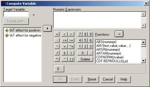
Select that your target variable (diff) is equal to pmsiat – nmsiat. Then click OK.
Now, run the
ANALYZE / COMPARE MEANS / ONE SAMPLE T TEST
command again. This time, your test variable is “diff.” You will get the following:

Notice that this is the same t, with the same dfs, significance level, and confidence intervals as when you ran the paired-samples t test.
Independent-samples t test: Now, let’s get a new data set that applies to independent groups.
In this study, the IAT is again used, this time to assess automatic associations with “mother.” The variable of interest is gender; that is, do males and females differ in their automatic associations with their mothers?
Ho: μmales =
μfemales. The
alternative hypothesis is H1: μmales
≠ μfemales.
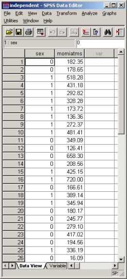
The data set is as follows (click here for the data set):
Notice
that you still have two variables, but here the first variable is the
independent variable (sex) and the second is the dependent variable
(momiatms, or a measure of automatic associations to “mother.” This
should look quite different from the paired-samples t test; put simply,
nothing is paired in this study. To run this t test, select: ANALYZE / COMPARE MEANS / INDEPENDENT-SAMPLES T TEST The
dialog box that you will get follows below.

Your test variable (the DV) is momiatms; the grouping variable is sex. You need to define the groups, which are 0 and 1 (what the experimenter has used, but you can use anything; here 1 is male and 0 is female).
Once you click OK, you will get the following:


Not much is new here; Levene’s test is a measure that tests an important assumption of the independent-samples t-test; that is, the two groups have equal variances. Here we’ll assume that the variances are equal (use the first line in the second table for your t).
What can you say about this study? It looks like your t, with 24 degrees of freedom (N1 + N2 – 2), is –2.084. The p-value is .048. You can reject the null hypothesis at the alpha level of .05, but what do you conclude? It appears that males have more positive automatic associations with “mother” than females.