In order to begin the design process, we needed to collect data. This is discussed in detail in Chapter 3. However, a few items are extremely relevant to the road design. Those items are listed below:
n Bill Traub’s road and setting design
n 10-meter DEM
n 1”: 400’ contour map
We were provided with an initial design performed by Bill Traub. This design included a complete road system, setting design, and PLANS analysis. Traub’s design covered a much larger area and was less detailed than ours.
We were provided with a 10-meter DEM. This did not provide us with enough resolution to perform the detailed analysis that we desired to perform. In order to have an adequate model of the terrain, we used a 1”: 400’ paper contour map. We printed our other coverages on transparent Mylar paper and overlaid them on top of the paper contour map.
From these maps, potential landings were identified on flat areas on the ridges (See Section 7.0). The next step in the design process was to design roads, on paper, to connect these landings to existing roads and to each other in a logical fashion. This process is called "pegging in" the roads. A divider was used to determine the desired grade and peg the road in between the control points, landings and existing roads. The guidelines used for this process are outlined below.
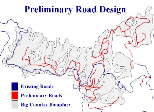
One important aspect of our design is the redundancy of some of the designed roads. Looking at the preliminary design in Figure 11, it is clear that there are more roads than necessary. This allows the flexibility to choose the best route from a range of options while in the field.
6.1.1 Side Slope Considerations
We developed a map coverage of side slopes and used this in the preliminary road design process. Whenever possible we tried to avoid pegging a road across a potentially unstable slope. The HCP states that all roads constructed on side slopes in excess of 40% must be designed with a full bench road prism. On roads with side slopes between 40%-55% a full bench road prism is required, but the excess material can be sidecast and compacted. Any road that is constructed on side slopes over 55% must have a full bench road prism and any excess material endhauled to a suitable disposal site.
On all roads constructed on side slopes of less than 40% a balanced cut/fill road prism may be used.
6.1.2 Road Grade and Alignment
Favorable road grades are defined as the downhill travel of a loaded log truck. Truck performance, safety, and DNR road standards limit the favorable grade to 18%.
Adverse road grades are defined as the uphill travel of a loaded log truck. Truck performance and DNR road standards limit the adverse road grade to 18%. There were some grades run at 18% to catch ridges or to stay on ridges. By doing this most wet areas and streams were avoided. We felt it would be better to sacrifice grade for location. The minimum curve radius used in the preliminary design of horizontal curves was 60 feet.
6.1.3 Stream Crossing
Recall from Figure 11 that we avoided stream crossings whenever possible by keeping the roads on the ridges. Most of the streams are located in incised channels that run north-south through the planning area. As you can see, most of our preliminary design avoids these areas. Our final design will cross even fewer streams.
Our fieldwork consisted of 4 weeks on the Olympic peninsula. During this time we set grade line, set P-line, traversed all of our designed roads, and ran corridor profiles. The data we gathered was then taken to the office and used to create the final design.
6.2.1 Processes
While performing field reconnaissance, when possible, the design team would follow the paper plans. The first step in locating the planned roads is to establish a grade line using orange flagging. Usually the grade line followed the paper plan very closely, however, there were areas where the paper plans needed to be modified in the field. These modifications were due to the need to avoid a problem area, due to changes in the desired ending point or due to the elimination of landing locations. For these areas, the design team would go ahead to the desired ending point, and then worked backward to miss the problem area until the flag lines met. The second step is to set a P-line with stakes. The last step is to perform an accurate road traverse of the P-line including distance, slope and side slopes.
6.2.2 Equipment
We used 3 different methods of traversing. The most basic was with a staff compass and chain. This was more tedious than other methods but provided consistent and accurate results. The method most familiar to this class was to use a Criterion impulse laser. This allows for multiple types of readings to be taken at one time and for them to be digitally recorded. The newest method to this class was using a LaserTech impulse laser, MapStar digital compass, and a Hewlet Packard data recorder. This method is fully automated and records all data that is needed for a traverse. Since this was a new instrument to the class several hours were spent learning how to operate the machine. Refer to the FE Handbook (http://courses.washington.edu/fe450) for detailed instruction on the operation of these instruments.
6.3 Field Reconnaissance Prioritization
Due to only a four week period in the field, time spent on road systems had to be allocated in such a way that areas of top priority were looked at first. We spent the majority of our time focusing on roads. Richard Bigley, in charge of DNR research and monitoring, identified this area for his research project. We prioritized the roads into 2 categories, primary roads and secondary roads.
During the three weeks of preliminary office work, primary roads were designed to access large areas within the timber sale. These roads were given top priority during the field reconnaissance since the road network was highly dependent upon the construction of these roads.
Some spur roads were pegged in on the maps in the office but were omitted from the gradelining and traversing done while in the field. These roads were given a low priority due to time constraints.
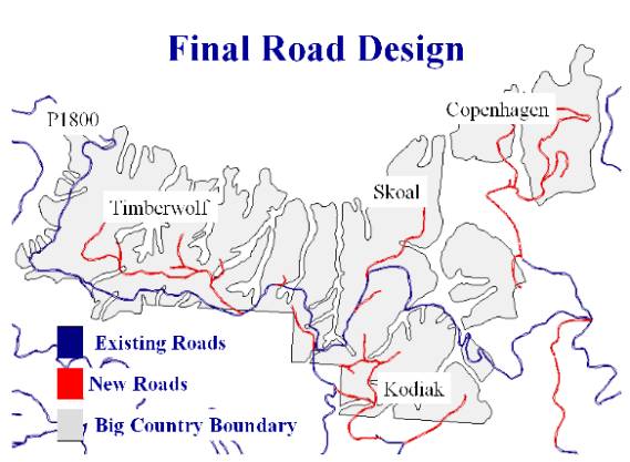
Our final road design reflects changes that were made after verifying our design in the field. This was created after visually analyzing road locations in the field and going through a RoadEng computer analysis in the office. Notice in Figure 12 that the final design is broken into five systems.
6.5.1 Road Statistics
Listed below are some summary statistics for the road design. The majority of roads that we designed were close to $2000 per station. However, there is one road that costs closer to $3000 per station. This is due to an extremely large amount of cut that has to be dealt with on a mainline road.
n Total designed road length: 11.8 mi
n New road length: 7.1 mi
n Reconstruction length: 4.7
n Cost per station: $1700 - $3000
n Access area: 1108 acres
We divided our road system into 5 groups. The group outlined in blue in Table 6 is existing road and our analysis accounts for its reconstruction. The rest of the roads are new roads.
|
Group |
Road |
Grade Range % |
Length (sta) |
Cost ($) |
|
P1800 |
P1800 |
0 – 15 |
329+50 |
639,502 |
|
South Road |
0 – 5 |
8+68 |
20,885 |
|
|
Kodiak |
Private |
0 -20 |
37+90 |
148,933 |
|
Kodiak |
0 - 16 |
41+50 |
86,478 |
|
|
Kodiak Ice |
1 - 17 |
9+45 |
17,623 |
|
|
Skoal |
Skoal |
0 -17 |
36+60 |
79,552 |
|
Timberwolf |
Timberwolf |
0 -16 |
69+10 |
208,880 |
|
West Rooster |
1 - 16 |
4+65 |
9,045 |
|
|
Copenhagen |
Copenhagen Black |
4 - 18 |
25+26 |
50,547 |
|
Copenhagen |
0 -15 |
71+99 |
164,217 |
|
|
|
|
Total |
63468 |
1,426,662 |
Ideally the maximum grade on any road would not exceed 15%. However we found that the best design sometimes required a grade up to 20%. Table 1 shows a breakdown of the road lengths and grade ranges.
6.5.3 Preliminary vs. Final Comparison
33. As you can see by comparing Figure 11 with Figure 12, there were some significant changes between the preliminary and final road designs. Most of these can be accounted for by the selection of better locations from multiple options while in the field. In the field we noticed things that had not been noticed on the map. Our extensive preliminary design allowed enough flexibility to easily work around almost all of these trouble spots. One noted exception is Rooster Road, located almost directly in the center of the map in Figure 11 (the ‘M’ shaped road). In the field, this road was found to be infeasible with no alternative routes.
There are four main challenges for road design in the Big Country Timber Sale. The first is the east bridge over Cougar Creek. Second is the west bridge over the Clallam River. Next is the south access. The final challenges are alignment issues. The road alignment changes on three roads, depending on which access route is chosen.
6.6.1 Big Country Road Design Specifications
Road design proceeded according to the following design criteria:
Design Vehicle: Log Truck
Critical Vehicle: Yarder
Design Speeds:
Main = 25 mph
Spur = 10 mph
Traffic Service Levels
Main = C
Spur = D
Traveled Width
Main = 12’
Spur = 10’
Slopes:
Fill Slope: 1 ½:1
Cut Slope: 1:1 => on steeper side slopes you may want to decrease to ¾:1
Ballast & Surfacing: 1 ½:1
Ballast Depth: 12”
Surfacing Depth: 12”
Curve Widening(added to inside of curve)
DNR specs:
2 feet extra --- 80 to 100 foot radius
4 feet extra --- 60 to 80 foot radius
USFS specs: go to
http://courses.washington.edu/fe346/projects/bridge_99/curvewidening/PS2.xls and use the excel sheet to calculate the widening based on the USFS equation
Fill Widening
Based on fill height at shoulder
<6’ => 2’
>6’ => 4’
The widening for fills <6’ is flexible. As the height of fill decreases, the widening can decrease, i.e., 1’ of widening for a 3’ fill.
Turnouts: put one in about every 1000 feet. You can also put them in tight curves as part of curve widening.
50’ length
12’ width
50’ taper each side
Much of the road design for the sale is straightforward. The major roads follow ridges, with spurs as necessary. The following sections detail the major challenges faced in designing the roads for the Big Country Timber Sale.
6.6.2 East Bridge (Cougar Creek)
The main challenges at the east bridge are the area itself, fill and curve widening, and the bridge design.
6.6.2.1 East Bridge Area
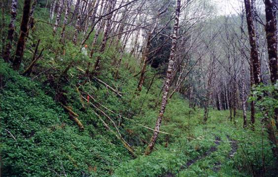
The east bridge area is characterized by geologic instability, wet areas, primary vegetation of alder and salmonberry, and steep side slopes.
Areas of geologic instability are identified in Susan Shaw’s “Geo” Arc/Info coverage and those identified by Wendy Gerstel on aerial photos and through field work. The east bridge has a deep-seated landslide associated with it as one of these unstable areas.
We recommend reading Wendy Gerstel’s pending final report on slope stability analysis for her conclusions on the stability of the area and recommendations on ways to mitigate the risk of road failure.


The steep side slopes make for difficult horizontal and vertical alignment. The road has to run at 18 percent for a ways just to maintain a ten percent grade through the s-curve towards the bridge. Even so, the road ends up having a through cut in a wet spot with a small stream.
6.6.2.2 Widening
Further, due to the alignment, a large quantity of fill is required in the s-curve (about 18 feet maximum). This through-fill is problematic because it makes curve widening a much larger issue than on a typical self-balanced prism. On a typical self-balanced prism, a ditch can be used as part of the curve widening, which adds about 3 feet to the road width. Thus, the DNR specification of four feet of curve widening for curves having a radius between 60 and 80 feet makes sense. However, with the through fill there is no ditch of which to take advantage. This, combined with the generally unstable soils in the area, necessitates that curve and fill widening be examined closely.
Also, one of the critical parts of this area is the bridge approach. The curves have to have enough widening at the bridge and also have a straight enough approach such that a log truck can pass it. Further, the widening at the approaches directly influences the width of the bridge over Cougar Creek. With that in mind, three approaches towards widening were examined. These were the DNR specifications, the curve widening equation, and the use of the drafting vehicle simulator. The following tables illustrate the results.
|
Method |
FW (ft) |
Lane Width (ft) |
CW (ft) |
Total Width (ft) |
|
DNR |
4 |
12 |
4 |
20 |
|
Curve Widening Equation |
4 |
12 |
6 |
22 |
|
Drafting Vehicle Simulator |
4 |
12 |
7 |
23 |
|
Method |
FW (ft) |
Lane Width (ft) |
CW (ft) |
Total Width (ft) |
|
DNR |
4 |
12 |
4 |
20 |
|
Curve Widening Equation |
4 |
12 |
6 |
22 |
|
Drafting Vehicle Simulator |
4 |
12 |
5 |
21 |
If there were no fill and hence, no fill widening, then the curve widening values would be four feet greater. For example, if there were no fill at the widest point on the s-curve, then the following results would occur:
|
Method |
Lane Width (ft) |
CW (ft) |
Total Width (ft) |
|
DNR |
12 |
4 |
16 |
|
Curve Widening Equation |
12 |
10 |
22 |
|
Drafting Vehicle Simulator |
12 |
11 |
23 |
6.6.3 West Bridge (Clallam River)
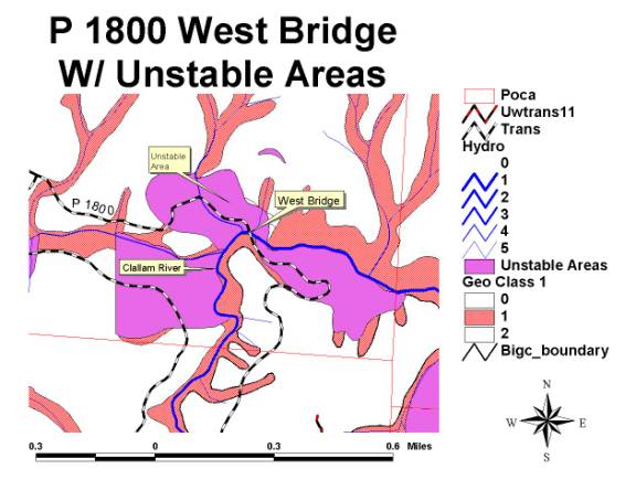
The major issues at the west bridge of the P1800 are road stability and the need to replace two major culverts. The bridge replacement itself should be fairly straightforward as a site survey was conducted in 1984. This survey was included in the project’s deliverables to DNR.
In the west bridge area, the P1800 cuts through a head scarp for about 300 feet. Other than this section of road, however, much of the road in the area is built on unstable ground. As Figure 17 shows, geologic instability in the form of shallow-rapid and deep-seated landslides dominate the area, including the bridge site. Cut and fill slope failures, slumps, steep side slopes, and several springs all characterize the area.
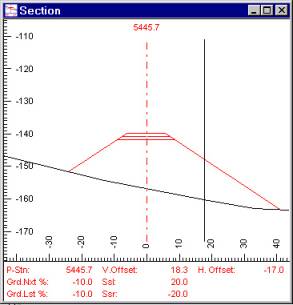
Because of the instability of the area and steep side slopes along the road, it would be a good idea to use some reinforcement technique to prevent the cut bank from failing. See the RoadEng cross-section printouts for more details on the cross sections.
As well, we recommend reading Wendy Gerstel’s final report (pending) on geology and slope stability for her analysis results.
![]()
6.6.3.2 Culverts
There are two major culverts west of the bridge that need to be replaced. Both are on large streams that empty into the Clallam River.
The one closest to the bridge is currently 72 inches in diameter and is a candidate for an open bottom or arch culvert. The other is 60 inches in diameter.
6.6.3.3 Site Survey
A bridge site survey was conducted at the west bridge in 1984. We entered the survey notes into a software package from TDS called Foresight to put them into electronic form. These files are included on the project CD in the transportation section.
In 1987, a geotechnical survey was conducted at the bridge site. The report provides extensive geologic notes for the bridge area, as well as recommendations on excavation and footings.
During the fieldwork phase of the project, we also reestablished some of the benchmarks at the bridge.
6.6.4 South Access
The south access eliminates the need for bridgework for this timber sale and also allows us to avoid building through unstable areas. However, it will need a substantial amount of work in order to meet Forest Practice standards. It needs realignment in at least one location in order to deal with sloughing of the cut and fill slopes. This will result in a large amount of excavation to deal with the steep cut slopes. It also needs about 19 new culverts, and 17 of the existing culverts need to be upgraded to larger diameters.
Given the road’s current location and condition, it represents a need for continuous maintenance, as well as a required easement. However, there may be a better option.
6.6.5 Southeast Access
In the Clallam Landscape Plan, Bill Traub designed several roads through the Big Country Timber Sale. Most of our roads closely follow his designs, and one of these is a road that will bypass much of the South Access. We flagged in this bypass road, but it still needs to be traversed. The advantage of this road is that it is located on a ridge for its length, reduces the amount of work the south access alone represents, and has the potential to decrease the amount of easement required over the Crown land.
6.6.6 Alignment
Some adjustment of road alignment will have to be done depending on what access route is chosen. The east access affects the alignment of Skoal and Kodiak Ice. The west access affects only Timber Wolf.
6.6.6.1 East Access
Skoal takes off east from the P1800 as currently designed. Coming from the east, however, necessitates that Skoal’s takeoff be changed to head NNW. There is a gradeline flagged in along this direction and is ready to be traversed. However, this area is problematic because the slopes coming off the P1800 here are very steep (60-70%). Thus, it is difficult to get the needed grade separation to get away from the mainline quickly or at a grade less than 15%.
The access to the landing at the end of Kodiak Ice will have to be changed as well. Its current design comes off the P1800, but the only other way to the landing is off one of the Kodiak spurs. There is a gradeline that was flagged in from Kodiak as far as the saddle before the landing, but was taken out of consideration early in the fieldwork. The current design was deemed more practical.
6.6.6.2 West Access
If the west access is chosen, only Timber Wolf has to have its alignment changed. In its current design, the road is set up for an east access. To come from the west requires that a switchback be added to the beginning of Timber Wolf. Adding in a switchback brings the road back to what Bill Traub had originally planned for it.
6.6.6.3 South Access
All of the roads were designed for a south access, so no alignment changes are necessary.
6.7.1 Introduction
The purpose of the access analysis was to evaluate 5 possible access routes by comparing the roads as they lead from the centroid of the planning area to a common point. The common point to compare all the routes was the Main gate to the P1800 just off Highway 112. This makes it possible to compare the 5 access routes objectively because all the routes start at the same point and end at the same point. From this, the distances were extracted and broken into speed zones in order to calculate the haul time out of the project area. In addition to haul time and subsequently haul cost, major direct costs of rebuilding the access routes were considered. The result is the total cost attributed to hauling 18200 MBF to the end point of the comparison while factoring in the costs to adequately reconstruct each access road up to the planning area boundary. By evaluating the costs from two fixed points the best route can be determined as the access with the lowest overall cost. This method should also be used in conjunction with other known design intangibles to make a precise access choice. Figure 24 is a conceptual representation of the planning area and access routes.
Northeast Southeast East West West Bridge Bloedel Planning Boundary for Big Country
Timber Sale Crown Gate Main Gate at Hwy 112 Cougar Bridge P1000
South
XXXX
P1800
East
Figure 24. Conceptual representation of the planning area and access alternatives.
6.7.2 Haul Cost and Reconditioning for each Alternative Access
6.7.2.1 Haul Cost
To calculate the haul cost between the two common points, the haul time for the duration of the project had to be determined. The first step was to isolate and extract the total distances of each route from the transportation GIS layer with ArcView 3.2 software. These access distances were then crosschecked on the maps we had of the area. The next step was to identify the speed a logging truck would be traveling at different locations along the access until the truck reached Highway 112. The first pass was conducted in the office by utilizing aerial photos, GIS orthophotos, GIS transportation layers, the GIS DEM of the area as well as existing maps. The aerial photos and orthophotos were used to look at the surrounding condition and alignment of each access. The DEM was then utilized to extract basic grades. Segments were then classified into speed zones using the basic grades, alignment and condition of the roads. These speed zones are described in Table 10.
|
Speed Zones |
|
Description |
|
|
12 mph (poor) |
Draws and Switchbacks, More difficult grades |
||
|
18 mph (moderate) |
Better Alignment, still difficult grades |
|
|
|
25 mph (mainline) |
Mainline roads better grades and alignment |
||
|
40 mph |
Paved mainline |
|
|
|
50 mph |
Paved Highway |
|
|
Once the speed zone distances are found and allocated the haul time can be calculated. Using distance equals rate multiplied by time, each speed zone time was determined then summed for the total time out to the main gate. A total haul cost could be projected by taking into account round trips, amount of volume being extracted, a logging truck payload of 4 MBF, and a truck rate of $60/hr. See Table 11 for results of haul costing to the mill.
Table 11. Haul Costing for each access to the Mill
|
HAUL Variables |
UNITS |
East |
West |
NE* |
South* |
SE |
|
12 |
mph Zone (miles) |
5.54 |
5.47 |
4.06 |
4.82 |
4.43 |
|
18 |
mph Zone (miles) |
0.4 |
0.7 |
0.95 |
2.35 |
2.34 |
|
25 |
mph Zone (miles) |
0 |
4.48 |
0 |
0 |
0 |
|
40 |
mph Zone (miles) |
0 |
3.25 |
0 |
0 |
0 |
|
50 |
mph Zone (miles) |
17.7 |
17.7 |
17.7 |
17.7 |
17.7 |
|
Total Distance |
miles |
23.64 |
31.6 |
22.71 |
24.87 |
24.47 |
|
Total Time to get out |
minutes |
50 |
67 |
45 |
53 |
51 |
|
ROUND TRIP |
minutes |
101 |
133 |
89 |
106 |
102 |
|
Total Haul Time For Project |
minutes |
457487 |
605608 |
406831 |
483877 |
465829 |
|
Total Haul Cost |
$ |
$457,487 |
$605,608 |
$406,831 |
$483,877 |
$465,829 |
6.7.2.2 Reconditioning Costs for Each Access
The reconditioning costs for the access roads considered extraneous costs particular to each access such as reconstruction, new construction, abandonment, maintenance, easements and bridges. Cost per station estimates were obtained through Bill Traub who provided the Western Washington Costing Estimates for Comparing Construction, Maintenance, and Abandonment, whichclassifies the estimates $/station as high, medium or low. The classifications were defined by gradient combined with sideslope classes. This includes abandonment and bridges inside of the planning area where applicable. All maintenance 1-year totals were multiplied by 5 to represent a 5-year road life. All abandonment cost scenarios are derived from portions of the P1800 that do not have to be reconstructed, but do incur the cost to close (See P1800 Scenarios for locations). Bridge costs were obtained through Eric Carlsen.
n EAST – The east access has a 55 foot bridge span estimated at the highest range possible at $3000 per foot yielding $165,000 due to design issues for the Cougar Creek bridge approach. The East bridge area consists of 85 stations, all of which were allocated the largest maintenance rate at $37 per station. The rest of the east access received a medium classification of $18 per station. The reconstruction for the East access is minimal because the P1800 has the costs for reconstructing the Cougar Creek bridge.
n WEST – The west access has a 100 foot bridge span estimated at the average range of $2500 per foot yielding $250,000 bridge total. An extra $20,000 was allocated to the bridge cell because of the need for a 6-foot diameter culvert to cross another stream. All maintenance for the west approach was given a medium classification leading to the planning boundary. No major reconstruction is needed for the access (West Bridge costs are reflected in the P1800 scenarios).
n SOUTH – The south access does not necessitate a bridge but the south access is owned by two private owners and does require an easement purchase. The easement is based on approximately 950 attributing acres. An estimated $125,000 for an easement was determined through consulting Aaron Roark, an Olympic Region engineer. Through field reconnaissance, we also evaluated the level of reconstruction necessary on the south access. The south access was deemed a high classification of reconstruction at $900 per station, which totaled $240,000. Connecting the South access with the P1800 would take some new construction, but this is evaluated in the P1800 scenario.
n SOUTHEAST – The southeast access is very similar to the south access. It differs by an addition of about 85 stations of new road on easy ground. At $1850 per station the new segment of road would cost about $128,000, in addition to necessary reconstruction totaling $126,000. The southeast access also proceeds onto private land for a shorter length than the south access. The easement would total about $96,000.
n NORTHEAST – The northeast access has been ruled out upon field verification due to slope stability, terrain and proximity to multiple fish bearing streams.
The total haul and reconditioning of the access alternatives is listed below.
|
RECON. COSTS |
UNITS |
EAST |
WEST |
NE |
SOUTH |
SE |
|
Easement Cost |
$ |
$0 |
$0 |
$0 |
$125,636 |
$95,899 |
|
Maintenance Distance |
miles |
4.44 |
8.65 |
5.12 |
7.17 |
6.77 |
|
Maintenance Cost x 5yrs |
$ |
$35,751 |
$38,821 |
$22,979 |
$32,179 |
$30,384 |
|
Reconstruction Distance |
feet |
6200 |
0 |
0 |
26769.6 |
14040 |
|
Reconstruction Cost |
$ |
$34,100 |
$0 |
$0 |
$240,926 |
$126,360 |
|
New Construction Distance |
feet |
0 |
0 |
3650 |
0 |
8400 |
|
New Construction Cost |
$ |
$0 |
$0 |
$73,000 |
$0 |
$128,100 |
|
Road Abandonment Distance |
Moderate STA |
35 |
47 |
82 |
82 |
82 |
|
Road Abandonment Distance |
Difficult STA |
24 |
26 |
26 |
26 |
26 |
|
Road Abandonment Cost |
$ |
$7,470 |
$8,910 |
$12,060 |
$12,060 |
$12,060 |
|
Bridge Cost (est. $2100-3000/ft) |
$ |
$165,000 |
$270,000 |
$200,000 |
$0 |
$0 |
|
Total Cost For ACCESS |
$ |
$692,338 |
$914,429 |
$702,809 |
$882,618 |
$846,572 |
|
Total $$/MBF |
$ |
$38.0 |
$50.2 |
$38.6 |
$48.5 |
$46.5 |
6.7.3 Internal Road Scenarios for the P-1800
The P-1800 is the existing mainline road inside of the Big Country Timber Sale Boundary. This road has 3 basic scenarios depending on which alternative access is chosen. The three scenarios reduce the 323 station total length of the P-1800 based on road that does not need to be reconstructed and can subsequently be abandoned because the timber sale will not justify its need. The locations and lengths are as follows.
Figure 25. P-1800 Reconstruction/Abandonment Scenarios
IF WEST:
P-1800 will not necessitate the East Section reducing the P-1800 from 323 stations to 221 stations. The road would be located coming from the east to the west from stations 112+00 to 327+00. Cost for adjusted P-1800 = $499,437.
IF EAST:
P-1800 will not necessitate the West Section reducing the P-1800 from 323 stations to 264 stations. The road would be located coming from the east to the west from stations 0+00 to 264+50. Cost for adjusted P-1800 = $500,605.
IF SOUTH or SOUTHEAST:
P-1800 will not necessitate the West or East sections reducing the P-1800 from 323 stations to 162 stations. The road would be located coming from the east to the west from stations 112+00 to 264+50. Cost for adjusted P-1800 = $315,564.
6.7.4 Internal Road Costs
The final components of the total access costs are the individual costs of each proposed road stemming from but not including the P-1800. Costing out each road was achieved by gathering quantities of total surfacing, total ballast, total end haul, culverts, and clearing and grubbing square footage (achieved through RoadENG data sheets). From these quantities we priced everything out the East Access. The Ballast and Surfacing component of the cost sheet required haul through a particular direction, thus east was chosen. The total road cost is comprised of six components. The six components are Clearing and Grubbing, Excavation, Ballast and Surfacing, Culverts, Geotextiles and Overhead (Costing Spreadsheets are located on the CD in the transportation section). All the accesses have the same internal costs except the South and Southeast, which have an addition of one major realignment particular to those chosen accesses.
IF WEST:
Cost = $766,217
IF EAST:
Cost = $766,217
IF SOUTH & SOUTHEAST:
Cost = $638,227
6.7.5 Total Overall Costs per Alternative Access
The final overall road costs for each alternative access consists of hauling the timber to the mill, rebuild cost, P-1800 cost and the internal road network.
These totals are estimates for each access. The internal road cost is the component that yields the most bias. Through time restraints it was not possible to cost each internal road particular to each access. All internal roads were cost evaluated to the east, which makes a difference in terms of surfacing haul costs. In addition, all roads were given geotextile in order to reduce the need to haul surfacing. This proves beneficial or breakeven to each access except to the east. Since the internal road network was evaluated to the east there is a $41 per station differential that should be accounted for in favor of hauling the surfacing.
IF EAST:
Cost = $1,959,218*
*There is $41 per station difference that needs to be accounted for because of the addition of geotextiles to the internal road network. Therefore, the east access needs to subtract $23,812 from the overall total to account for this discrepancy (Approx 11 miles of road). Adjusted total = $1,935,406
IF WEST:
Cost = $2,180,141
IF SOUTH:
Cost = $1,985,701
IF SOUTHEAST:
Cost = $1,949,655
6.7.6 Decision Matrix for Alternative Access
The following is a decision matrix that describes the intangibles of each access. The three main intangibles that could not be quantified in terms money are slope stability, design difficulty and Marketability. Slope Stability risk should be considered when making an access choice because of the large amounts of unstable soil and potential landslides in the area. Wendy Gerstel, DNR geologist, is finalizing the geological report of the area. Design difficulty should be considered because of alignment issues that would have to be observed for each access. Marketability is in reference to the purchaser and the sale ability for each access. The table below should serve to supplement the overall costs of each access in order to make an access decision.
|
159. |
160.SLOPE STABILITY RISK |
161.DESIGN DIFFICULTY |
162. |
|
163. 164. |
165. 166. High |
167. 168. High |
169. 170. Low |
|
171. 172.WEST 173. |
174. 175.Medium |
176. 177. Low |
178. 179. Medium |
|
180. 181.SOUTH 182. |
183. 184. Low |
185. 186. Medium |
187. 188. Medium - High |
|
189. 190.SOUTHEAST 191. |
192. 193. Low |
194. 195. Medium |
196. 197. High |
6.8.1 Introduction
Ballast and Surfacing is the most significant percentage of total cost to each road because of the long distance to the rock source. In an attempt to reduce the required 12 inches of surfacing to less than 12 inches we looked at introducing a geotextile that would make up the loss of structural integrity brought upon by reducing the surface material. After speaking with Brenden Reall, a representative of Contech Inc., a construction products distributor located in Port Orchard, the recommendation was to use a Tensar Earth Technologies Geogrid*. The TX1100 is a geosynthetic made from polyethylene that serves to distribute the load caused by wheel-to-road contact. Brenden Reall supplied us with SpectraPave Software version 1.2 to evaluate the subgrade for improvement. The program takes into account volume use, native base soil classification (CBR values), ballast material, surfacing material, and asphalt if necessary. The program results in a strength value. We first obtained a strength value with 12-inch shale ballast –12 inch 11/2 minus crushed surface, and a native soil CBR value of 4. With this given strength value we could now introduce the TX1100 and reduce the surfacing until we matched that strength value. Through the program, we reduced the necessary surfacing to 8 inches.
*Fabric was not considered because it does not add strength necessary to reduce surfacing to the road, it simply prolongs the road life.
6.8.2 Cost Comparison
In order to make a cost comparison we broke down the cost per station of 12 inches of surfacing and the cost per station of the TX1100 geogrid with 8 inches of surface. For a mainline there is 52 cubic yards needed per station with 12 inches of surfacing and 34 cubic yards with 8 inches. The TX1100 was quoted at 1.95 per square yard fully installed and required an additional foot on each side of the 12 foot running surface width. The results in Table 14 are tailored to each access because of varying haul distances.
6.8.3 Results
The east access is short enough that hauling the 12 inch surfacing is less costly than introducing the geogrid. The west is a good canidate for the geogrid and the south could offer some relief if other costs and intangibles are being considered as well. In the other scenarios and possibly other timber sales where haul is even longer, the Tensar TX1100 geogrid remains a viable option to reduce surfacing volumes.