Figure 3. Map of DNR’s structural stages.

Figure 4. Distribution of structural stage classes as a percentage of total acreage.

As a surrogate for these structural characteristics it is put forth that age may be used. Ages (in years) for the seral stages are defined as: Open: 0 - 10; Regeneration: 10 - 20; Pole: 20 - 40; Closed: 40 - 70; Complex: >70; and Fully Functional: >150. Using this results in the following distribution across the landscape (Figure 3). The closed structure dominates the landscape (88%) with small percentages of other structural stages (pole: 4% - fully functional: <1%). This can be further seen in the distribution of acreage for each structure (Figure 4). With the majority of the landscape in the closed structure provides many opportunities for harvesting to provide revenue to the trusts as well as move the stands into other structural classes.

Figure 5. Map of dominant species.

Figure 6. Standing Scribner volume to 6" top (mbf) by structural class. Of the total volume, Douglas-fir accounts for the largest fraction, 76%, with western helmock making up 12% and a combination western redcedar, red alder, bigleaf maple, black cottonwood and western white pine making up the remaining 12% (Figure 7)

Road density has traditionally been used as an index for planning future designs and abandonments. It is common practice to simply dismiss areas with high densities as ‘bad’ and areas with low densities as ‘good.’ However, density is oftentimes not the best gauge of a road’s potential impact to streams, etc. Frequently, in evaluation of potential impact the road’s proximity to streams is often overlooked and road density is substituted, many times to the disadvantage of a landscape manager. Therefore, it is good practice to evaluate road systems based on their location in the landscape rather than solely on density.

Consider the following argument. Sediment filtration occurs as overland flow travels downhill. The greater the distance traveled the more sediment filtered. This is the fundamental knowledge that today’s wider riparian buffers are at least partially based on. With the addition of adequate cross-drains and good road design the majority of water can be diverted to flow onto the hillside as opposed to down the road. Consequently, roads further from streams have less potential impact. This is true whether we are talking about roads further up on the hillside away from streams or about segments further from stream crossings, regardless of locale. The knowledge is nothing new and is the basis behind the movement to design hilltop roads and minimize the number of stream crossings a road has.

As a baseline for our analysis and to facilitate comparisons in our designs we still calculated the current road density. We challenge you to break the status quo and consider each design based on its innovation rather than simply dismiss it as being ‘good’ or ‘bad’ based on a common index. This is an important point because, the area we planned currently has a density near 3 mi/sect² which is the mandated cutoff for road density, designated by the District manager. Therefore, using the road density as a surrogate would virtually eliminate any road building in this area.

Road density is commonly reported in miles of road per square mile of land or per section (i.e., mi/mi² or mi/section). That convention is followed in this report. In conversations with DNR authorities the current road density was estimated to be about 1.5 mi/sect². The target density ‘not-to-exceed’ was mandated as 3 mi/sect². The following analysis was done to determine the actual baseline (current) road density given the data provided.

The total Hoodsport planning area was essentially split into two parts with the 1999 FE seniors responsible for the north and W. Jaross responsible for the south. The distinction needs to be made to help identify the derivation of the numbers used in the following analysis. The area used in our calculations was based on DNR property north of Jorsted Road also termed the ‘north Hoodsport planning area.’ Initial road lengths were based on roads provided in the DNR’s TRANS coverage.

The north Hoodsport planning area had approximately 46.2 miles of road in the coverage provided. Of this, approximately 3.1 miles is designated, as ‘trail’ but were more likely ‘railroad grade.’ The total area was determined to be approximately 16.4 square miles including small landholdings within the boundary.

The southern boundary of our planning area was the Jorsted Road. Consequently, the length of the Jorsted has to be considered in calculations density calculations of both the north and the south because technically it is in both. We chose to handle the Jorsted in the following manner. In order to assure it was not mistakenly counted twice in the calculations only one-half its length was used in density calculations for the north. Conversely, one-half the length should be used in density calculations of the south.

The length of Jorsted Road was estimated to be about 3.4 miles. One half of this is 1.7 miles. Therefore, the length of road used in calculating road density for the north is 46.2-1.7=44.5 miles.

The next decision was whether or not to include roads classified as ‘trails.’ If included the total road length remains 44.5 miles. If not, the total length of road is reduced to 44.5-3.1=41.4 miles. With these values in mind, the initial road density ranges from 2.5 mi/mi² (not including trails) to 2.7 mi/mi² (including trails).

It is important to note that the total area for the north was not amended to account for non-DNR landholdings within the planning area. It is very likely that these will become DNR property in the future alleviating the need for their special consideration. Furthermore, accounting for these tracts of land now would serve to decrease the overall area and to increase the overall initial road density of our planning area.

It is also important to note that the DNR coverage allows for classification of road types into several categories including roads, trails, railroad grades, etc. The density value is dependant upon which classes are included in the analysis. For example, you get a different value if you are using ‘roads’ as opposed to using a combination of ‘roads’ and ‘trails.’ The ‘road activity’ attribute, called ROAD.ACT.STAT.CD is also of no help because most arcs are coded as ‘99’ or ‘unspecified.’ The rest are coded ‘0’, which has no apparent equivalent in the data dictionary.

Another important note is that the value is only as good as the data. While we were in the field we noticed numerous old roads and railroad grades that were not included in the TRANS coverage. These would normally be included in the density calculations. However, since they were not in the coverage they were not used in the calculations.

During the project analysis we were provided access to a DNR wildlife biologist who helped us to identify what Marbled Murrelet habitat was. Therefore, we could identify it if we found it in the field. Generally, we were looking for ‘platforms’ that were up to 50 feet high and had a minimum 7-inch diameter of space. Platforms could be large branches of old-growth trees or dead tops of trees. These provided the perch that Marbled Murrelet desire. Near Dynamite Ridge there was a high concentration of snags that would lend itself to Murrelet habitat. Therefore, that area was given special attention in our analysis.

Stream modeling was generated for the Hoodsport planning area to aid in identification of many of the smaller streams not mapped within the GIS coverages. The original GIS Hydro layer was created using USGS 7.5’ quads and digitized from orthographic photos.

The DNR hydro layer did not contain many of the smaller streams that become important for analysis of sedimentation production potential and delivery in road location and design and slope stability issues. Road location and stream crossings were minimized during the planning with ridge location for road placement set at a high priority, but with better stream mapping, proper road designs at known crossings can help to reduce the impact of the road system on the hydrology of the watershed.

Three stream layers were created using ArcGrid analysis. Two models were derived to identify areas where water would most likely be located based on topographic information from USGS 7.5’ quads and DNR contours. Potential stream layers were modeled from stream power and flow accumulation. Stream power is based on the upstream flow length and gradient of the slope. Flow accumulation identifies areas of convergence by using the topography to determine the direction of flow from one cell to another and accumulates the volume entering each cell from above. A minimum limit or threshold was set for each method for identification of the stream network. The flow accumulation stream model was created with a minimum of 100 contributing cells from above to locate the beginning of a stream. This limit can be raised or lowered to compute a lower or higher density stream network respectfully.

Two models were chosen and placed on field maps, flow accumulation from USGS quads and DNR contours. These two stream networks can be seen in Figure 9. Stream power models were not chosen to be field verified because of the inconsistency in some areas. The stream reaches flowing through low gradient areas lost enough power and disappeared, leaving gaps in the stream network. It was thought that these would be good indicators of wetlands, but when compared to the other models and the DNR hydro layer, it nevertheless appeared to be too inconsistent. The USGS flow accumulated stream network was chosen because of its alignment with the DNR hydro layer and the DNR flow accumulated was chosen because of its alignment with the contours. Both models contained some parallel streams that when converted to a coverage, mutated into a lattice of lines which may be another indicator of wetlands.

Figure 9. The DNR DEM derived stream network atop the USGS DEM derived stream network for the Hoodsport planning area.

During the field verification portion of the project, many planned roads were gradelined with notes and many inactive roads were walked and inventoried. After the field verification was completed, the streams that were crossed during gradeline location and road inventories were identified on the stream model maps. The model that appeared to be most accurate was the DNR contour derived streams.

Figure 10. Legend for items mapped in stream figures.

Some of the stream crossings noted during the field verification are highlighted in the following figures. A legend for the items located on the figures of the various stream networks from Arc/Info is shown in Figure 10. The base layer is the DNR contours (each contour line is 100 feet) shown in gray. The transportation layer, including UW proposed routes is shown in dashed black. The hydro layer supplied to us by the DNR is shown in dark blue. The two stream networks analyzed from the field, DNR derived stream network and USGS derived stream network, are shown in red and purple respectively.

The image shown in Figure 11 is the FS-11 road. This road connects the UW proposed bypass for the slide on the Jorsted road to the U.S. Forest Service 2480 road. The circled areas are road inventory identified streams. The circled stream in the middle is a DNR derived stream that aligned with the DNR provided hydro layer unlike the USGS derived stream. The stream identified in the small circle to the left in Figure 11 does cross the FS 2480 in the depicted location, but does not actually cross the FS-11 road. This is probably due to the microtopography that the digital elevation matrix (DEM) can not portray in the cell size.

Figure 11. FS-11 road inventoried stream crossings. Circled streams were identified during the inventory activity.

Six streams were crossed on the FS-14 road inventory. Two existed on the DNR hydro layer, while the two known crossings and four unknown crossings were identified on the DNR derived stream network. Figure 12 shows three circled stream locations identified on the DNR derived stream network, while the USGS derived network identified two inaccurate crossings.

Figure 12. The DNR DEM-derived stream network is shown in red and the Hydro layer stream network in purple. Three of the six stream crossings identified during the road inventory of the FS-14 that were not shown on the Hydro layer but were predicted by the new stream network.

During the gradeline of the Waketickeh East (WM-1311) road and the gradeline and traverse of the Powerline road (WM-134) many additional streams were crossed that did not show up on the DNR hydro layer. The circled areas identify these streams from the DNR derived network.

Figure 13. The DNR DEM-derived stream network (red) over-estimates the actual number of streams by about 25 percent.

During the gradelining and road inventories, any streams that were crossed were recorded in the notes. Based on the number of predicted stream crossings from the DNR derived network and the streams that were recorded in the notes, an average and weighted average was produced for the model. The results from the road inventories and gradelines can be seen in Table 3. The accuracy in our model averaged 74% in stream prediction for the traveled areas.

Table 3. Prediction results from road inventoried and gradelined stream locations. The predicted number of stream crossings were tabulated from the field maps according to the number of streams that were predicted to cross a road. The actual number of streams that were crossed were noted and compared back to the field maps. Percent of prediction is the number of stream crossings divided by the predicted number of stream crossings.

UW-Road Name	Predicted Number of Stream Crossings	Actual Number of Stream Crossings	% of Prediction
FS-11	4	2	50
FS-14	10	6	60
FS-1462	1	0	0
J-2	12	8	67
J-23	6	5	83
J-2322	3	2	67
K-13/K-13RR	14	11	79
WM-1311	9	7	78
WM-134	16	14	88
		Average Prediction	63.6%
Weighted Average Prediction			73.6%

The initial prediction rate calculation was based on the actual number of stream crossings vs. the predicted number of stream crossings. This average prediction rate of 64% was skewed due to the proposed road FS-1462. The model only predicted one stream for this area, therefore the prediction would rate 100% or 0%. Because of this, we calculated a weighted average of 74% based on the total number of streams crossed to the total number of predicted streams to be crossed during the gradeline and road inventories.

Prediction of streams using this model is more accurate in high gradient and incised topography than in low gradient and flat topography. This is due to the microtopography that exists on the ground and does not show up on the DEM. The streams generated by the ArcGrid analysis flow in the direction of lowest gradient. The small fluctuations on the ground are not visible in a 30 x 30-foot cell, leaving it up to the smoothed depiction of the ground to dictate the flow path. Additionally, the derived streams are smoothed out to reduce the number of parallel streams that appear. This process also alters the location of the streams in the model.

The flow accumulation threshold of 100 was used to generate the stream models. This threshold could be lowered or raised. Lowering the threshold would allow the streams to start further upslope than the streams created with the threshold at 100. This would also increase the stream density. Similarly, raising the threshold would create streams that began further downslope and lower the stream density. Field verification would be needed for any limit chosen for the initiation of a stream.

Our stream model can be used to estimate increased cost for additional stream crossing culverts on planned roads that have not been gradelined or traversed. Additionally, sediment delivery can be estimated more closely with the additional stream crossings that exist. This estimate, however, may be slightly higher than what may be delivered due to the possible inclusion of additional stream crossings.

Stream preservation and water quality has become a high priority for land managers. The two main contributors to the sediment transported through the stream network are hillslope surface erosion and sediment generated from roads. The amount of sediment that is generated from these two processes is an important factor in the movement of sediment to the streams and stream protection, however the primary concern is the amount of sediment that will be delivered to the streams.

Surface erosion from hillslopes is generated from soil creep and the erosive potential of water. Soil creep is active at all times. It is the slow movement of soil downslope due to gravitational forces and other biological situations such as the burrowing from animals and falling trees. Additional surface erosion is generated when soil particles, especially those located on slopes of higher gradients, are not protected from the impact of rainfall and then to overland flow. These two forces and mass wasting events are the natural transport mechanisms for soil entering stream networks. Figure 14 shows a mass wasting event on the Jorsted road delivering sediment to the stream network. Unlike soil creep and potential mass wasting events, erosion from rainfall and overland flow rarely occurs on forested lands. A thick, absorbent organic layer or duff protects forest soils from rainfall unless a management activity such as harvesting or road building removes this protective layer.

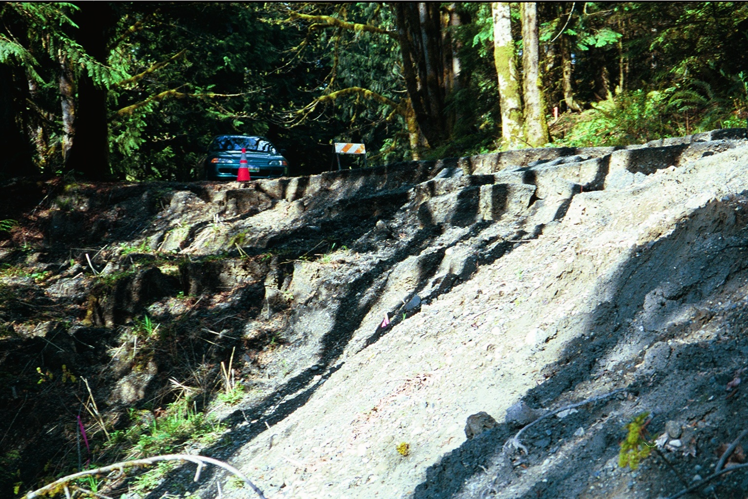
Figure 14. Mass wasting event on the Jorsted road delivering sediment to the stream network.

The amount of vegetation present will also affect the sediment delivery into streams. Given enough distance and vegetation between the point of sediment generation and the stream, a filtering of the sediment may occur, temporarily reducing the actual amount of sediment that will be delivered. However, there are many factors that affect the timing of natural sediment production that enters the stream including the proximity to streams, slope angle and soil particle size and amount of vegetation available for filtering potential.

Road construction and use is another major sediment source in a managed watershed. Construction of roads removes the vegetation, exposing the mineral soil layers, adding to the sediment generation in the area. 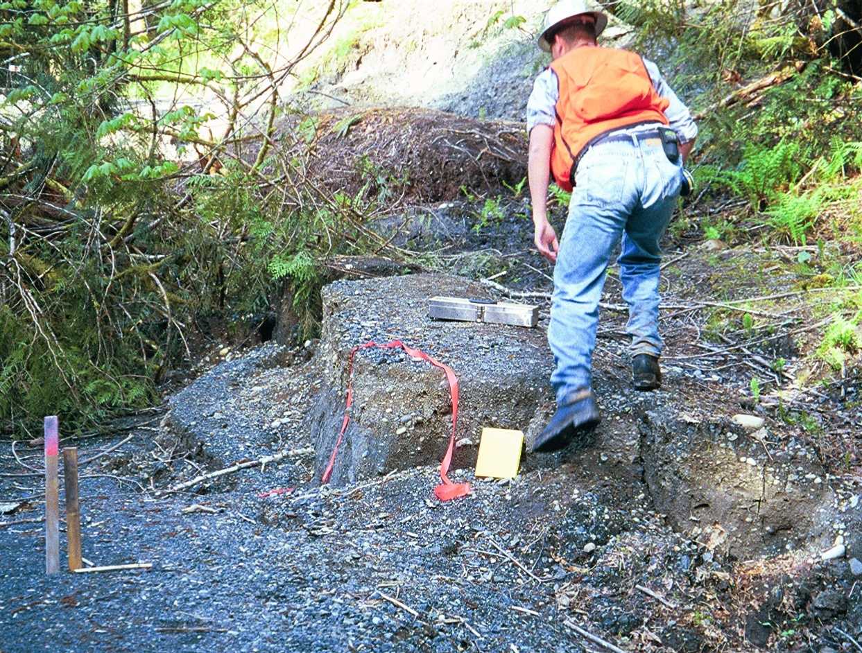Once the road is established, the cutslopes and fillslopes will revegetate, reducing the sediment production from the previously exposed soil, although the ditch and tread will continue to be a source of sediment production. Figure 15 shows an eroded road surface and fillslope delivering sediment to the stream network below due to a poorly maintained ditch. The amount of delivered sediment generated by road segments are affected by the length of road that delivers directly to streams, materials used for surfacing, and use levels on the road segments.

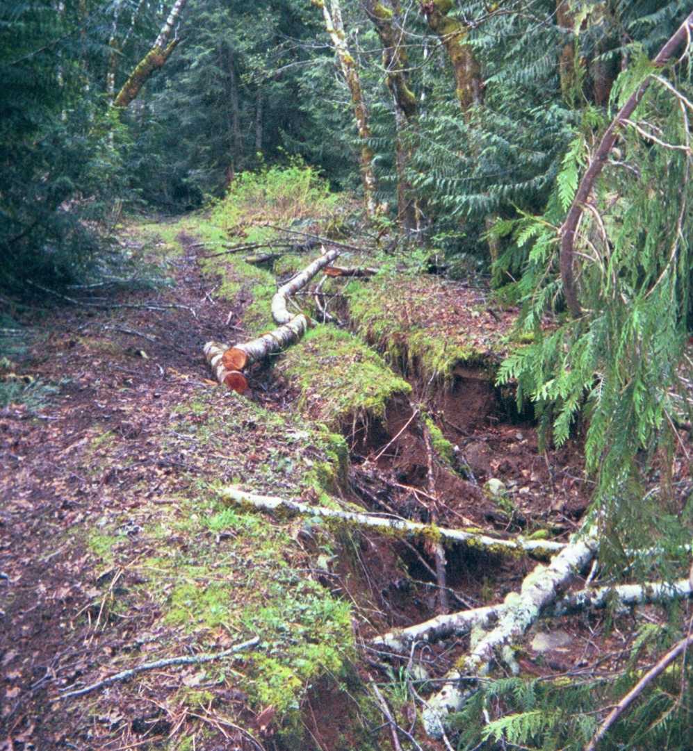
Figure 15. A Full ditch diverted water down a road bed, eroding the road surface and eroding into the fill slope, delivering sediment to the stream below.

For the Hoodsport planning area, we used a GIS based road erosion/delivery model developed by Boise Cascade Corporation. This model aids land managers in identifying road segments with a high potential of delivering sediment to streams within the watershed. The road erosion model is based on the Washington Department of Natural Resources Standard Method for Conducting Watershed Analysis surface erosion module (WDNR 1995), with some modifications (SEDMODL-Boise Cascade Road Erosion/Delivery Model, Technical Documentation 1999). A few assumptions were used in the development of this version of the model. It is assumed that all roads are older than 2 years old and all roads are in-sloped with a ditch. Furthermore, if the stream or road layer is off spatially, then the amount of road and stream intersections has the potential to increase the amount of direct delivery road segments or decrease the amount of direct delivery road segments, consequently affecting the amount of sediment delivery potential.

The surface erosion module uses the width of the various road prism components in combination with the following items to determine the road erosion potential:
Parent Material to determine the Basic Erosion Rates
The Surfacing Material to determine the Surfacing Factor
Level of Use / Road Class Category and Annual Precipitation to determine the Traffic and Precipitation Factor
Road Length
Vegetation Factor

Once the erosion potential is determined for each segment of road, the model determines the road sediment delivery areas. These areas are identified by the proximity of roads to streams. The road network is divided into three categories: stream and road crossings that will deliver 100% of sediment generated, roads within 100 feet to 200 feet that will deliver a portion, 35% and 10% respectively, of the sediment generation but not directly to the stream and other road segments that will not deliver to the stream network.

The background sediment input is calculated from the stream channel length, soil depth, average soil creep rate and soil bulk density. This amount of sediment input into the stream network can be used to compare the amount of sediment input from roads to the amount of sediment input from natural processes in determining whether roads are having a major effect on the water quality of the streams.

Output of this model will provide:

Estimated Total Road Sediment (including a breakdown of tread and cutslope sediment)
Estimated Road Sediment per Mile
Total Background Sediment
Road and Background Sediment Ratio
Length of Direct Delivery Length

We used this model in the Hoodsport planning area for estimating the amount of sediment production and delivery potential to streams. The model was run on the existing roads with a comparison of the two hydro layers, the DNR provided hydro layer and the DNR derived streams that was created by the UW. Within the program, many parameters need to be defined. Road width, road use and road surfacing need to be assigned from the coded transportation layer for sediment generation and delivery to streams. Additional items that are more specific to the area also need definition. Included are soil depth (average), the soil's average bulk density, minimum and maximum soil creep rates and a percent vegetation cover for cutslopes generalized for the area. An example of the values used in the model for the existing roads can be seen in Figure 16.

Road Class Item Value Road Width Road Use

====================================================

HIGHWAY 1 40 Moderately Heavy

PRIMARY 2 25 Moderate

SECONDARY 3 18 Light

SPUR 4 15 Occasional

ABANDONED/BLOCKED 0 12 None

Road Surface Type Item Value

=======================================

ASPHALT 1

GRAVEL 9,2

------------------------------------------------------------------

VARIABLES TO BE USED BY THE MODEL

------------------------------------------------------------------

Soil Depth: Model will use average depth (in) from soil coverage.

Bulk Density: 1.4 gm/cc

Min Soil Creep: 0.040 in/yr

Max Soil Creep: 0.080 in/yr

Cut slope cover: 60%

Figure 16. Variables used for road width, level of road use and road surfacing as well as the variables used for soil properties and vegetation of the cutslope.

  The estimated sediment from the DNR provided hydro layer is most likely lower than the true sediment production and delivery amount. This is primarily because the DNR's hydro layer does not contain many of the smaller streams that greatly affect the sediment delivery amount from background sediment and roads causing a lower than normal amount for sediment production and delivery. The results from the sediment model (SEDMODL) can be seen in Figure 17.

------------------------------

SEDMODL RESULTS

------------------------------

Total Estimated Road Sediment:...... 92 tons

Estimated Road Sediment per Mile:

(based on indirect delivery).…… 2 tons

Estimated Tread Sediment:.........…. 31 tons

Estimated Cutslope Sediment:......... 61 tons

Background Sediment Total:........... 1008 tons

Road/Background Sediment Ratio:. 0

Road Direct Delivery Length:......... 5.7 miles

Mean Cutslope Height:.............…... 7 feet

Mean Road Width:..................……16 feet

Mean Precipitation Factor:........…..1.01

Figure 17. Estimated road and background sediment for Hoodsport planning area using the DNR provided hydro layer and existing roads.

  SEDMODL also outputs new coverages identifying the road segments and their estimated sediment delivery amount that have potential to deliver to the stream network. This new layer can be seen in Figure 18 for the estimated sediment from existing roads and the DNR provided hydro layer.

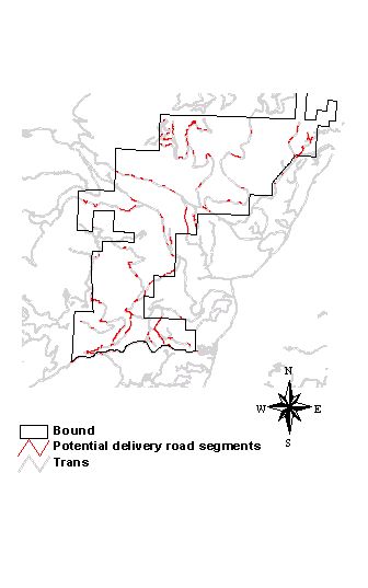
Figure 18. Road delivery segments (shown in red) for the existing roads and the DNR provided hydro layer from SEDMODL. The output ArcView layer includes sediment amounts for each segment.

The DNR derived stream network over-estimated the amount of streams that exist in the area creating much higher sediment potential and delivery amount. The derived stream network had a greater density than the DNR provided hydro layer and the actual ground. This created larger sediment totals than expected. Figure 19 shows the results of the sediment totals for the derived stream network.

------------------------------

SEDMODL RESULTS

------------------------------

Total Estimated Road Sediment:...... 272 tons

Estimated Road Sediment per Mile:

(based on indirect delivery).…… 3 tons

Estimated Tread Sediment:.........…. 112 tons

Estimated Cutslope Sediment:......... 160 tons

Background Sediment Total:........... 2479 tons

Road/Background Sediment Ratio:. 0

Road Direct Delivery Length:......... 45 miles

Figure 19. Estimated road and background sediment for Hoodsport planning area using the DNR derived stream network and existing roads.

  The identified road segments and their estimated sediment delivery amount for the existing roads and the derived stream network can be seen in Figure 20.

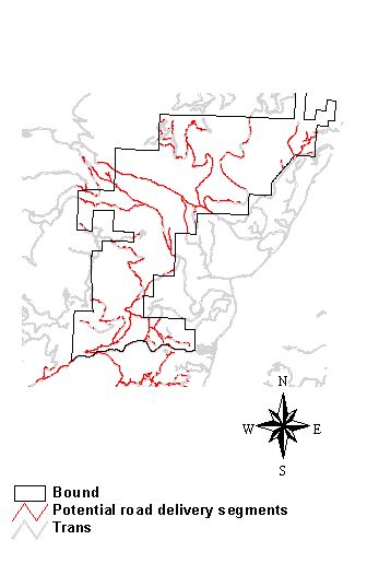
Figure 20. Road delivery segments (shown in red) for the existing roads and the derived stream network from SEDMODL. The output ArcView layer includes sediment amounts for each segment.

During the field verification portion of the project, stream crossings of gradelined and inventoried roads were noted and checked against the maps of the derived stream networks. Based on the stream verification of the derived network (Chapter 5.7.1), the sediment estimates calculated from this stream network will be amended according to the results of the verification process. The percentage of existing streams to the prediction of streams within the derived stream network was 74%. Using this percentage, all estimated SEDMODL results were reduced approximately 26%. This amendment changed the over-estimated results to lower numbers which are more likely to be closer to actual amounts but still are probably too high. The amended results can be seen in Figure 21.

---------------------------------------------

AMENDED SEDMODL RESULTS

---------------------------------------------

Total Estimated Road Sediment:...... 201 tons

Estimated Road Sediment per Mile:

(based on indirect delivery).…… 2.2 tons

Estimated Tread Sediment:.........…. 83 tons

Estimated Cutslope Sediment:......... 118 tons

Background Sediment Total:........... 1834 tons

Road/Background Sediment Ratio:. 0

Road Direct Delivery Length:......... 33 miles

Figure 21. Amended estimate for road and background sediment for Hoodsport planning area using the DNR derived stream network and existing roads.

  Results from the SEDMODL on finalized UW proposed roads within the Hoodsport planning area can be seen in Chapter 14.

The slope stability analysis for the Hoodsport planning area was generated with the Shaw Johnson model. This model identifies unstable slopes by the curvature and gradient of the topography. Table 4 shows the curve classes used for this model.

Table 4. Slope classes used in the Shaw Johnson slope stability model. Low, Moderate and High are associated risks within each category.

Slope Class
Curvature	0 - 15%	15 - 25%	25 - 47%	47 - 70%	> 70%
Concave	Low	Low	Low	Low	Moderate
Planar	Low	Low	Low	Moderate	High
Convex	Low	Moderate	High	High	High

Past landslides were identified on aerial photographs. These areas were digitized to analyze the topography associated with these landslides. Once the landslides were digitized, ArcGrid was used to correlate the landslide locations with curvature and gradients to develop the classes for Table 4. The gridstack, a feature within ArcGrid, shows the curvature, gradients and identified landslides against one another. This correlation can be seen in Figure 22. An image of the Shaw Johnson stability model for the Hoodsport planning area can be seen in Figure 23.

Figure 22. A screen capture from ArcGrid showing the curvature, gradients, and landslides plotted against each other.

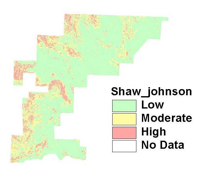
Figure 23. Shaw Johnson stability map for the Hoodsport planning area.

This type of stability model is useful as an initial stability analysis, however there are more variables that are attributed to a failure. Better analysis would be obtained using the infinite hillslope equation and factor of safety, however the input variables for this analysis include many soil properties that was not available for the soils in the planning area.

Conversations with the DNR geologist suggested some other areas to look at. Within the soils layer provided by the DNR, a wasting potential attribute existed. A wasting potential of 3 or 4 indicated moderate to high potential for mass wasting. These two wasting potential classes in combination with headwaters of streams would help in identifying areas with wasting potential and steepened slopes due to incision. In order to find the location of headwaters, the UW derived stream network was used. Using the Strahler ordering system, our streams were segmented. Using the 1 and 2 Strahler ordered streams and the wasting potential classes of 3 and 4 from the soils layer, an additional stability map was created. This additional stability map can be seen in Figure 24.

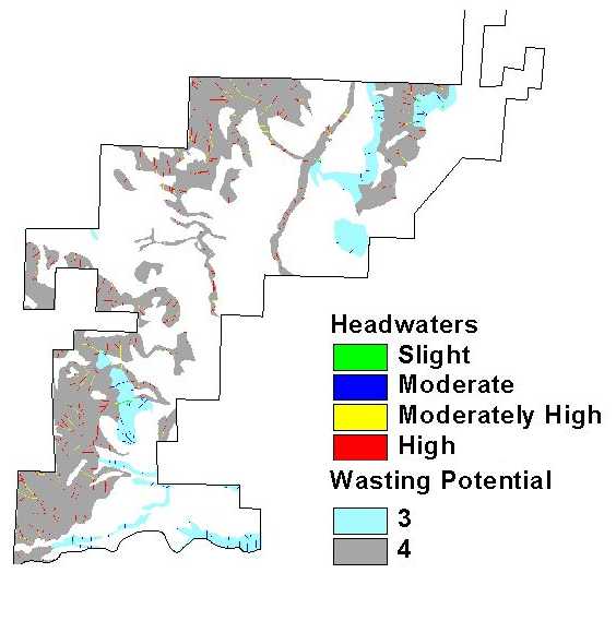
Figure 24. Stability map of wasting potential and headwaters of streams.

The areas of the headwaters with high and moderately high ratings correlated well with the Shaw Johnson stability map. Lastly, an area with minimal soil depth and an underlying restrictive layer of clay was another good place to look for instability. As discussed in the Stability Issues, Chapter 5.4, when there is a layer of clay underlying much of the soil combined with a low soil depth, water has the potential to create a layer for the soil above to slide upon. These two qualities, the clay and low soil depth within the planning area, also associated well with the Shaw Johnson stability map generated for the Hoodsport planning area.