Introduction to Geographic Information Systems in Forest Resources

UW Home GIS@UW Search

Syllabus Schedule Class Meetings Assignments Course Data Contact Us CFR 520 Lab Locations Software Collect It Page

Objectives:

• learn to use theme-on theme selections
• learn to use spatial joins
• learn to use tabular relates

1. Perform drive substitution to create drives L (CD) and M (removable drive).
2. Open a map document
3. Create an event layer from polygon centroids
4. Selecting points near a line
5. Selecting adjacent polygons
6. Line-on-polygon selection
7. Polygon-on-line selection
8. Point-in-polygon selection
9. Polygon-on-point selection
10. Polygon-on-polygon selection
11. Spatial join: containment (inside)
12. Spatial join: proximity (nearest)

Perform drive substitution

Perform drive substitution to create the virtual drives L and M.

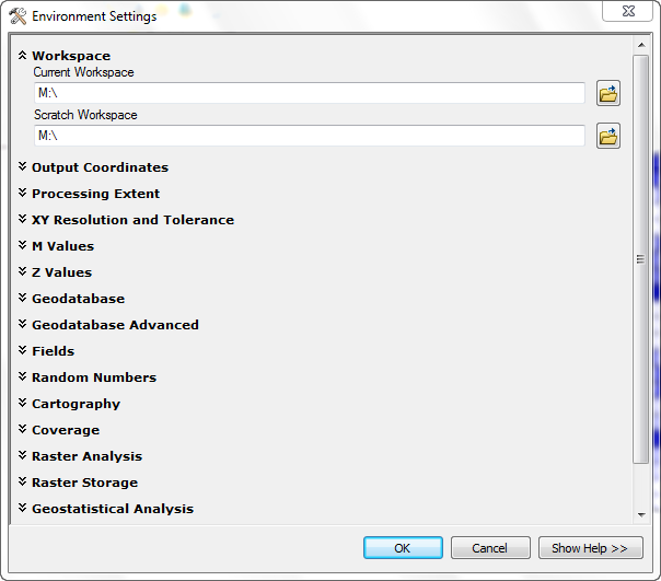
1. Open ArcMap and set the working directory to your M drive (Geoprocessing > Environments):
   
   
   
   
2. Download the map document v_an_1.mxd, and save it in this directory.
   
   
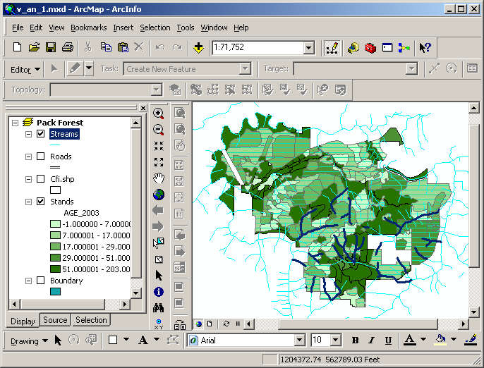
3. When the map document opens, it will appear with a data frame displaying Pack Forest.
   
   

Create an event layer from polygon centroids

We are interested in which continuous forest inventory (CFI) plot centers are close to streams, and what that distance is. There may be a relationship between amount of timber, species composition, etc. and distance to streams

However, for this exercise we only have a CFI polygon layer. Because we have the plots stored as polygons, we need to convert to points. This process will allow us to create a point dataset from the polygons.

1. Export the CFI layer to M:\NETID.gdb\cfi. Note that you will now have 2 CFI polygon layers in the map, one stored on the CD and the other on your USB drive. Make sure you can identify which layer is which.
   
   
2. Open the attribute table for the new cfi shapefile (the one stored on your removable drive).
   
   
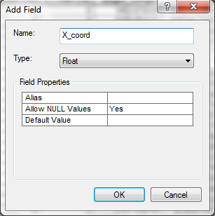
3. Add a field called x_coord to the table (Options > Add Field), following this format:
   
   
   
   
4. Add a field called y_coord to the table (Options > Add Field), following by same format.
   
   
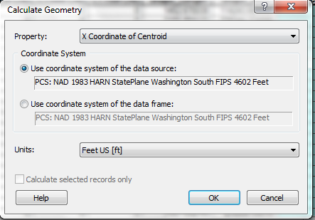
5. Right click the mouse from the top of x_coord/y_coord, then select Calculate Geometry ....
   
   
   
   
6. You may see the same warning message as above (if so, click Yes). The Calculate Geometry dialog will open. Choose the Property method X Coordinate of Centroid . Also make sure the upper radio button is selected.
   
   
   
   
7. Click OK. Now you should see the X coordinates of the centroid of each polygon has been added for each record. Do the same operation with Y coordinates, and then you will see the table like this:
   
   
   
   
8. Export the table to M:\NETID.gdb\cfi_centroid_table.dbf (Options > Export):
   
   
   
   
   
   Now the exported table is added to the map (see the Source tab).
   
   
   
   
9. Close the table.
   
   
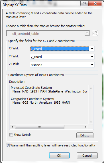
10. Right-click on the the new table in the Table of Contents and select Display XY Data.
    
    
    
    The dialog will automatically show the default X and Y fields.
    
    
11. Click the Edit button for changing the coordinate system of the new points.
    
    
    
    
12. Click Import (we will be importing coordinate system properties from the original CFI data set).
    
    
    
    
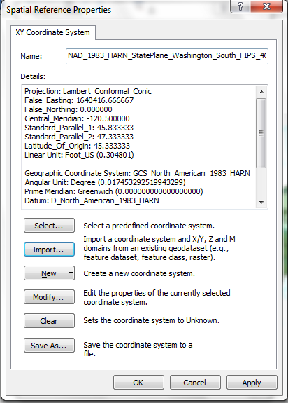
13. Double-click cfi to import its coordinate system properties.
    
    
    
    
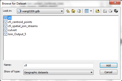
14. Now you will see the imported properties. Click OK.
    
    
    
    Click OK to add the points to the map
    
    
    
    
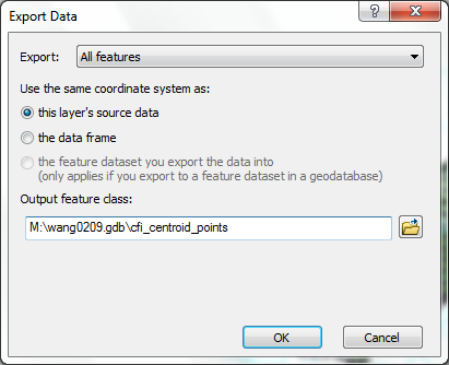
15. Now you will see the points display as "Events." Note that these point events are stored only in volatile memory. To create a permanently stored data set it is necessary to export the point events.
    
    
    
    
16. Right-click the new layer and Export to M:\NETID.gdb\cfi_centroid_points.shp.
    
    
    
    
    
    
17. You can now delete the exported CFI polygon layer and the exported table from the map, but keep the new CFI centroid points layer. We will use these points in the next section.
    

You just made a copy of the CFR polygon data, added X and Y coordinates to its table, created point events from those coordinates, and finally created a new point data set from the point events.

Method 1 (simple)

1. From the Selection menu, choose Select By Location.
   
   
   
   
2. Select features from cfi_centroid_points that are within a distance of features in Streams with a selection buffer distance of 50 feet, as shown:
   
   
   
   
3. Click Apply and then Close. The selected points are within 50 feet of a stream.
   
   
   
   While this method allows you to easily select features that are within a specified distance of features in another layer, it does not tell you exactly how far each feature is from the source.
   
   

Method 2 (more complicated, but more powerful)

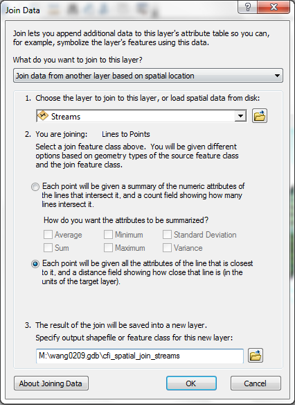
1. Right-click the cfi_centroid_points layer and select Joins and Relates > Join.
   
   
   1. In the first dropdown, select Join data from another layer based on spatial location.
      
      
   2. Click the radio button for Each point will be given all the attributes of the line that is closest to it, and a distance field showing how close that line is.
      
      
   3. Specify the output as M:\NETID.gdb\cfi_spatial_join_streams.
      
      
   4. Click OK.
      
      
      
      
2. Open the newly joined table. You will see all the attributes of the CFI points, along with the fields from the streams layer, and a new field called Distance. The values from the streams layer are those from the stream that was closest to each point. The Distance field, which is created automatically, contains the distance from each point to that closest stream line.
   
   
   
   
3. Open the properties for the cfi_spatial_join_streams layer and change the symbology to graduated color using the brown monochromatic color ramp based on the Distance field.
   
   
   
   
4. Turn off the stands layer for a better view.
   
   
   
   The darker plot centers are further from streams, and the lighter plot centers are closer to streams. Do you think the proximity to streams may affect the species composition of these plots? How would you find out?
   
   
5. Make a selection based on the Distance field:
   
   
   
   
6. Open the attribute table, show only Selected records, and then sort ascending based on Distance.
   
   
   
   While the selection of features is identical in the two methods, by using the joined distance field, not only do you get to select features that are within a specified distance, it is also possible to understand the distribution of the distances.
   
   
7. Richt-click the Distance field and select Statistics. The mean distance of plots from streams for those plots within 50 ft of a stream is 22.8 ft. (Due to some installation error, the lab computer will not be able to show the graph as the following figure, but you will be able to see it in the other ArcGIS installed computer.)
   
   

You have just performed several actions. First, you converted a polygon layer to a point layer by using the X,Y coordinates of the polygon centroids. This can be useful when you want to represent or analyze polygon data as a series of points rather than as polygons. Second, you joined a point attribute table and a line attribute table, creating a new point layer. This is a special type of join that always joins attributes of pairs of the closest features, and also automatically calculates the distance between each pair of features. A point-to-line spatial join takes advantage of the spatial relationship of proximity between features of separate layers.

This process will select only those stands that are adjacent to 70-80 year old stands (not including the 70-80 year old stands).

1. Open the Stands attribute table. Right-click the AGE_CLASS_2003 field and select Summarize.
   
   
2. The only summary statistic is AREA > Sum. Place the summary table in M:\NETID.gdb\stands_age_class.
   
   
   
   
   
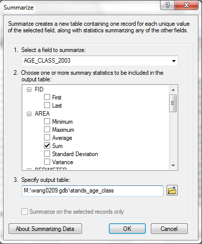
   This creates a table with a unique value for each 10-year age class, containing an additional attribute for the total area within each age class.
   
   
   
   
3. Perform a Relate (right-click, Joins and Relates > Relate) between this table and the original Stands attribute table, as shown below:
   
   
   
   
4. Select the record in Attributes of stands_age_class for 71-80 year old stands. To select records from the same age class from the Stands table and layer, click (in the .dbf table) Options > Related Tables > age_class : polygon.
   Note you could have performed this selection using a query, but you should get familiar with this alternate, and in some ways, more efficient, method of using summary tables and links.
   
   
   
   
   
   
   
   Now your selection includes those stands in the 71-80 year age class.
   
   
5. Next, perform a spatial selection to get stands that are adjacent to the currently selected set. From the menu, choose Selection > Select By Location.
   
   
   
   
6. You want to select features from Stands that intersect the features in Stands, as shown below:
   
   
   
   Apply and Close the dialog.
   
   
7. Next, in order to get a selected set of stands which are adjacent to those in the 71-80 year age class, but excluding those in the 71-80 year age class, from the menu, choose Selection > Select By Attributes. Your selection on Stands should Remove from current selection (use that Method in the Select By Attributes dialog) those stands which are in the 71-80 year age class.
   
   
   
   
8. Because the default selection symbol is a thick cyan outline, it is not possible to discern between selected polygons and those that are surrounded by selected polygons. We will alter the selection symbol now. Open properties and click the Selection tab for the Stands layer.
   
   
   
   
9. Double-click the selection symbol to open symbol properties. Choose a Line Fill Symbol.
   
   
   
   
10. Make sure to use the same color (any color you choose) for the Fill Color and Outline Color.
    
    
    
    
11. Now you can clearly see those polygons that are selected and those that are not.
    
    
    
    Your selection of stands includes those that are adjacent to the 71-80 year age class, but not including the 71-80 year age class.

You have just performed a selection of a group of spatial features based on their proximity to a different set of features. This can be useful when analyzing phenomena which are affected by proximity or adjacency. For example, if a pathogen spreads from one area to an adjacent area, you can use this to find possible locations of pathogen spread.

Which DNR Type 4 & 5 streams pass through young to middle aged stands?

1. Select young to middle aged stands (age < 40 in 2004). ESTAB_YEAR is the year of establishment for each stand. You will need to type in the year value 1964, rather than selecting from the list of values, since there are no stands established in 1964.
   
   
   
   
2. To make a selection of streams that pass through these selected stands, choose Selection > Select By Location. Make a selection from Streams that intersect with the features in Stands.
   
   
   
   Apply and Close.
   
   
3. Now reduce the selection of streams to only DNR Type 4 & 5 (Selection > Select By Attributes). Make sure to use the Select from current selection method.
   
   
   
   
4. In order to see the selected streams more clearly, change the selection symbol to a thick blue line:
   
   
   
   

You have just selected a set of linear features that traverse a set of polygonal features. This is useful when analyzing the relationship between linear features and their underlying polygons. For example, is the quality of road surface dependent on median household income per census tract? Or is the presence of salmon in a stream reach affected by the basal area per acre within a riparian management zone?

Which stands are traversed by tertiary roads?

1. Select all tertiary roads with a query on the Roads layer. Make sure to use the Create a new selection method.
   
   
   
   
   
   
2. Use Select By Location to select features from Stands that intersect the features in Roads, as shown below.
   
   
   
   
3. You can now see those stands that have at least part of a tertiary road inside the stand boundary.
   
   

This type of analysis is the reverse of the previous analysis. In this case, we are interested in what polygons may be affected by linear features. For example, which municipalities does a proposed regional light-rail traverse, or which forest stands may be affected by a diesel fuel spill in a large stream?

Which CFI plot centers are within soils with moderate to high windthrow potential?

1. Create a new data frame called Soil Data.
   
   
2. Add the L:\packgis\packgis.mdb\forest\soil as well as the M:\NETID.gdb\cfi_centroid_points.shp (created earlier) to this new data frame.
   
   
3. To make the different soil types visible, make a graduated color 6-class natural break classification on the Windthrow.cd field in the Soils attribute table.
   
   
   
   
4. Select moderate-to-high windthrow potential soil polygons (windthrow code greater than or equal to 3).
   
   
   
   
5. Select By Location to select CFI plot centers that are contained within moderate-to-high windthrow soils polygons. Make sure the use selected layers checkbox is checked (this will limit the selection of points to those selected soils polygons).
   
   
   
   
6. To make the selected set of plot centers more visible, clear the selected set of soil polygons (right-click on the Soils layer and choose Selection > Clear Selected Features).
   
   
   

You have just made a selection of points that are within a given set of polygons. This type of analysis is valuable when determining if point measurements are affected by the polygons in which they lie. For example, is the calculated density from a series of inventory sample points affected by the soil type from which the measurements were taken?

Which forest stands overlap with the selected set of moderate-to-high windthrow potential CFI plot centers?

1. Make sure your selected sets for cfi_centroid_points are set to features with moderate-to-high windthrow potential from the previous section.
   
   
2. Copy the Stands layer from the to the "Pack Forest data frame" to "Soil Data data frame".
   
   
3. Use Select By Location to select stands that completely contain the selected set of plot centers, as below.
   
   
   
   
4. You can see how the overlapping stands are selected.
   
   
   
   
5. Turn off display of the plot centers in order to get a better view of the selected stands.
   
   
   
   This is a very cursory estimation of stands that may have moderate to high windthrow susceptibility. It is not completely reliable because a polygon containing even a single high-windthrow plot is flagged as "moderate to high" windthrow susceptibility. However, it could be used as a field reconnaissance map for investigating stands after a windstorm.

You have just selected a series of polygons that overlap with another selected set of points from another layer. This is useful in determining if there is a relationship between a point and a polygon layers. For example, is the species composition of forest stands in any way related to the sampled aspect class or soil type?

Polygon-on-polygon selection

Another way to approach the previous problem is to select forest stands that overlap with moderate to high windthrow soil types. Polygon-on-polygon selections are done in the same manner as the other layer-on-layer selections.

Here are a series of polygon-on-polygon selections as examples. Attempt each one of these. The layers used are Soils (with a selection of moderate-to-high windthrow polygons) and the Stands. The type of relationship is listed in bold. Note that in order to reproduce these, you would need to alter the selection symbol as shown below (to a diagonal line fill).

Stands that intersect selected soils polygons, This probably overestimates the number of stands.

Stands that are completely within selected soils polygons, This probably underestimates the number of stands.

Stands that completely contain selected soils polygons

Stands that have their centers in selected soils polygons

Which of these most closely represents "reality?" That is really a question for the resource specialist. The GIS can provide a number of different scenarios, but the ultimate decision must be made by a person who knows the resource.

The example of analyzing CFI plots based on the underlying soil type using layer-on-layer selections works well for a single query. However, this becomes tedious if you want to know which plots lie in several different soil types. This type of problem is better solved with the spatial join. In this case the spatial join will be between a point and a polygon layer, rather than a point and line layer in one of the previous sections.

1. Clear all selections (from the menu, choose Selection > Clear Selected Features). This clears all selections from any layer in the data frame, whereas right-clicking on a layer in the table of contents and choosing Selection > Clear Selected Features only clears the selection for that layer.
   
   
2. Right-click the cfi_centroid_points layer and select Joins and Relates > Join. Follow the example below to create a new point layer that will have the attributes of the soils polygon in which each point falls.
   
   
   
   
3. Make sure all selections are clear from the new point layer, then right-click the CD_27 field (previously WINDTHROW.CD in the soils attribute table), and create a summary table called M:\v_an_1\windthrow_basal-area.dbf, with the summary statistics BA1994CPA > Minimum, Maximum, Average and BA1994HPA > Minimum, Maximum, Average. This will create a new table with a record for each unique windthrow code value, along with a summary value of the minimum, maximum, and average basal area (BA) per acre per tree class (H = hardwood, C = conifer) in 1994 per windthrow code class.
   
   
   
   Add the new table to the map document.
   
   
   
   This table is a summary that was made from a joined field. There may be a pattern: plots with lower windthrow potential seem to have higher basal area. If soils have greater potential for windthrow, then more trees should get blown over, thus the basal area will be lower.
   
   
   
   
4. Perform a relate between the summary table and the points (note: where it displays CD below, use the CD_27 field):
   
   
   
   
5. Now selections on the windthrow_basal-area summary table are displayed on the data frame. (Remember, you could perform these selections using a query, but a relate makes the selections more efficient.)
   
   Windthrow code 0:
   
   
   
   
   
   After you select the row for CD = 0 click Option at the lower right of the table GUI and then select Related Tables > windthrow::soils. After this, you should see the points with CD = 0 also selected in the map display.
   
   Windthrow code 1:
   
   
   
   
   After you select the row for CD = 1 click Option at the lower right of the table GUI and then select Related Tables > windthrow::soils. After this, you should see the points with CD = 0 also selected in the map display.
   

You have just used the technique of performing a spatial join of a polygon attribute table onto a point attribute table. This adds to the point attribute table attributes for the underlying polygons. This is used for tasks such as determining the soil type for a series of vegetation plot samples.

Do plots closer to streams have a higher hardwood volume than plots farther from streams? Answering this may require some tricky table joining.

1. Add the Streams layer to the current data frame.
   
   
2. Perform a spatial join of the stands on the Join the Stands layer attribute table onto the cfi_centroid_points layer. This will append the attributes from the Stands layer to the CFI plot centers, creating a new point data set.
   
   
   
   Each plot center is coded with the attributes for the underlying stand polygon. We now know the forest type for each plot center.
   
   
3. Now join Streams onto the output of the last join:
   
   
   
   
4. Open the table for the output of this join and summarize the table based on the SPECIES field, with the summary statistic DISTANCE > Average.
   
   
   
   
5. Sort the output table in ascending order by Average_Distance.
   
   
   
   How do you interpret the species types in the CFI sample plots with the distance of the plots to streams? Do you expect this type of species-distance relationship given what you know about riparian vegetation? Remember that these species values are not the actual species measurements from the plots themselves, but rather the predominant species for the stand in which the CFI plots lie.

This technique is used to determine if spatial location (in this case, distance to streams) seems to have any relationship to the physical properties of the location. You could use this to help quantitatively answer the question: for a group of marbled murrelet nests, what underlying vegetation type is closer to streams or farthest from roads?

REMEMBER TO TAKE YOUR CD AND REMOVABLE DRIVE WITH YOU!!!!

Return to top

Syllabus Schedule Class Meetings Assignments Course Data Contact Us CFR 520 Lab Locations Software Collect It Page

The University of Washington Spatial Technology, GIS, and Remote Sensing Page is supported by the School of Forest Resources

School of Forest Resources