SURFACE EROSION MODULE
| ||||||||||||||||||||||||||||||||||||||||||||||||||||||||||||||||||||||||||||||||||||||||
 |
Method
Surface Erosion is primarily based upon the soil characteristics, the topography and water. The analysis will be in three categories hillslope erosion, erosion due to roads and streambank erosion or soil creep. The hillslope erosion and erosion due to roads can be analysed into erosion potential and delivery. Hillslope erosion is calculated using the Universal Soil Loss Equation or USLE. This equation was generated by the USDA for erosion on agricultural fields. Within our analysis the USLE was revised to be more applicable to forested settings by altering two of the variables within the equation. The road erosion potential and soil creep was based on the process outlined in the Watershed Analysis Manual (WAM).
Hillslope Erosion
Hillslope erosion is essentially a function of the soil characteristics, the topography and the vegetative cover. Within the analysis we will examine the potential for erosion, the effect of forest activities on the erosion potential and based on the proximity to streams, whether it will be delivered to the stream network. Whether the hillslope erosion will deliver to streams will be based upon the distance and slopes that the soil must travel. The hillslope erosion potential will be analyzed using the Universal Soil Loss Equation (USLE). The USLE equation is:
where, A = Tons / Acre / Year
K = the Soil Erodibility Index
S = the Slope factor
L = the Length factor
R = the Rainfall index
C and P = Management and Vegetative Factor
As discussed earlier the USLE was derived for agricultural land but this equation was revised or more specifically the C and P variable was revised to be more applicable to other settings including forested areas. For our analysis, the total tons/acre/year was revised to tons/year in the location where the sediment originated. The K factor was determined from the amended soil layer created for this project area. The slope and length factor was determined from the grid analysis on the dem. The rainfall index was determined from an article about the revised soil loss equation for the western United States. The C and P factor had two different values, one for the present forested condition from Dunne and Leopold, Water in Environmental Planning, and another for simulated harvesting (personal interview, Finn Krogstad). A value on 1 for P was used in both conditions for no erosion control practice while the C was varied. Forested conditions were assumed to have 0.003, where the harvesting areas used a value of 0.33 for slopes less than 30% where tractive logging could occur and slopes greater than 30% used a value of 1.00 for skyline logging.
Road Erosion
Road Erosion is estimated based upon the type of road, the road prism (road dimensions including the road width, length and slope of the cut and fill slopes), soil properties of the sub-grade, road surfacing type, traffic levels and precipitation within the basin and a correction for the amount of vegetation that has occurred on the cut and fill slopes. The road erosion potential as suggested by the WAM assigns a basic erosion rate to each componenet of the road prism which then becomes ammended for various properties specific to the roads in the Watershed Analysis Unit.
The road prism comonents and the percentage of surface erosion attributed to each component are:
- Road Tread = 40%
- Cutslope and Ditch = 40%
- Fillslope = 20%
The basic erosion rates are then determined by the parent material. Within our project area, the parent material was estimated to fall within the categories of High/Moderate, Moderate and Low from Table B-5 of the WAM depending on the soil parent type listed in the DNR soil coverage. Because the area has not been logged in quite sometime, the roads were estimated to be older than two years generating the basic erosion rates.
|
|
|||
|
|
|
|
|
|
|
|
|
|
|
|
|
|
|
|
|
|
|
|
|
|
|
|
|
For example, roads located in areas containing parent materials found in the Moderate category older than two years would be modified in this way:
- Road Tread = 40% of 30 = 12 tons / acre of road tread / year
- Cutslope and Ditch = 40% of 30 = 12 tons / acre of cutslope and ditch / year
- Fillslope = 20% of 30 = 6 tons / acre of fillslope / year
The next step is to correct the basic erosion rates for cut and fill slopes based upon the vegetation existing on the road component. In the Hoodsport area, the assumption was that the roads were old enough for the ground cover density to be equal to or greater than 80% leading to a correction factor of 0.18 from Table B-6 of the WAM. This will change the example cutslope and ditch erosion rate to 2.16 and the fillslope rate to 1.08.
|
|
|
|
|
|
|
|
|
|
|
|
|
|
|
|
|
|
|
|
|
The roads located in our project area were labeled as Type 4 roads. From the DNR data dictionary, a type 4 road is classified as an unimproved road for use during fair and dry weather. Based on this description, the assumption was that it was an old forest road surfaced with greater than 6" of gravel for the surface. According to Table B-7, the correction factor for the road tread component would be multiplied by 0.2 equating to a new erosion rate for the example road of 2.4.
|
|
|
|
|
|
|
|
|
|
|
|
|
|
|
|
|
|
Lastly, the erosion rates are amended for the amount of traffic on the roads and the average annual precipitation for the watershed analysis unit. Our basin and the surrounding areas averaged over 130 inches annually. According to table B-8 this would be in the last category, > 3000mm. Assuming that these roads would not be driven during the wet weather of the winters and have only light traffic for the rest of the year, the traffic and precipitation correction factor is:
1/4 * .1 + 3/4 * 1 = .775
|
|
|
||
|
|
|
|
|
|
|
|
|
|
|
|
|
|
|
|
|
|
|
|
|
|
|
|
|
The adjusted erosion rates for all road prism components in the example would be:
- Road Tread = 40% * 30 * 0.2 * 0.775 = 1.86 tons / acre of road tread / year
- Cutslope and Ditch = 40% * 30 * 0.18 * 0.775 = 1.674 tons / acre of cutslope and ditch / year
- Fillslope = 20% * 30 * 0.18 * 0.775 = 0.837 tons / acre of fillslope / year
Once the erosion rates have been determined, the amount or area of each component is multiplied by the rate to determine the total potential for erosion. A road width was estimated for the type 4 roads was assumed to be 12' and the area of the cutslope and fillslope was estimated from the Washougal 98 Project.
Delivery of sediment to the stream network was estimated by proximity to streams. If a road crossed a stream, 100% of the sediment flowing down the ditchline for 200' on either side of the crossing would be delivered. This would include sediment generated by the cutslope, ditch and road tread assuming the road is insloped. When determining the delivery potential, roads segments that cross the streams for 200' were added to the stream network when determining the delivery areas. Sediment generated from the fill slope would be estimated at 10% reaching the stream for roads located within 200' of the streams. Roads not within 200' of the stream network would be assumed no delivery.
Streambank Erosion
Streambank erosion or soil creep, is estimated by the WAM using stream length, slope, creep rate, soil depth and fraction of fine grained soil sizes. The soil depth and fraction of fine grained soil sizes was found within the DNR soil coverage for the area. Stream length and slope were found with grid functions using the dem. The creep rate was estimated in the WAM:
A = L * 2 * D * C * F
where, A = Annual Erosion Volume (m^3 / yr)
L = Stream Length (m)
D = Soil depth (m)
F = Fraction of Fine Grained Soil Particles (%)
C = Soil Creep Rate (m / yr)
- If average slope is less than 30%, the creep rate = 0.001 meters / year
- If average slope is greather than 30%, the creep rate = 0.002 meters / year
For comparison to the other sections within the surface erosion module, the streambank erosion was converted to US Customary Units.
Results and Discussion
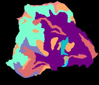
The hillslope erosion was estimated by the USLE. Two simulations were used to predict potential soil erosion, the first simulation was for present vegetated conditions and the second was to simulate harvest operations within the area. The hillslope potential for both situations can be found in figures 2 and 3. Areas chosen for harvest were stands age 50 years or older. This was an arbitrarily chosen age. Areas where the stands were 50 years or older accounted for approximately 1/3 or the entire project area and were located on both lower and higher gradient slopes for better comparison.
Figure 2. Hillslope erosion potential for present vegetated conditions. Units for the legend (upper right corner) are in tons / year. |
Figure 3. Hillslope erosion potential for simulated harvest operations. Units for the legend (upper right corner) are in tons / year. |
Both situations had increased hillslope erosion occuring in the steeper sloped areas of the basin, but the magnitudes are quite different. In the completely vegetated situation with no logging occuring, the most amount of sediment generated over the course of a year is 11% of a ton where as in the second situation, the greatest amount of sediment generated where logging was present was on the order of 35 tons. This was estimated assuming no erosion prevention was utilized in the logged areas for an example of a more extreme situation.
The road erosion potential was estimated by following the Watershed Analysis Manual's approach to sediment generation from roads. Sediment generation was computed for each component of the road prism. Our basin contained primarily one road type, type 4, which is an unimproved road for use during fair to dry weather and a small portion of a road type 0 which is a trail as classified in the DNR data dictionary. The surface erosion potential for each road component was based on the soil parent material, vegetative cover, road surfacing materials, traffic and precipitation. Figures 4,5 and 6 show the amount of erosion potential for each component in tons / year.
|
|
Figure 5. Surface erosion potential for the cutslope and ditch in tons/year. |
Figure 6. Surface erosion potential for the fillslope in tons/year. |
As expected, more sediment was generated within the cutslope/ditch and road tread areas than the fillslopes, but unexpectedly, the amounts generated were less than the hillslope sediment potential in the present vegetated situation.
Delivery potential was determined by a 200' distance of a road near a stream. Figure 7 is a picture of the roads and streams within the project basin.
Figure 7. Roads and streams located within the project
basin.
|
|
When determining the delivery area and delivery potential, roads crossing streams were added to the stream network since 100% of the sediment transported through the ditch would be delivered to the stream network. Fillslopes located within 200' of the stream network would be expected to deliver 10% of the sediment generated from this road prism component. Figure 8 shows the delivery areas and percentage of sediment delivered as a function of distance.
Figure 8. Delivery areas and percentage of sediment
delivered as a function of distance.
|
|
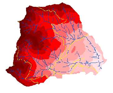
The sediment generated by the hillslope erosion and the road erosion was combined within the delivery distance to determine the amount of sediment that could be deposited into the stream network. The amount of sediment delivered to the stream for the present vegetated situation can be seen in figure 9 and the harvested situation can be seen in figure 10.
Figure 9, Hillslope and road sediment delivered to the stream
network for the present vegetated situation.
Figure 10. Hillslope and road sediment delivered to the stream
network for the harvested situation.
|
Figure 9, Hillslope and road sediment delivered to the stream network for the present vegetated situation. |
Figure 10. Hillslope and road sediment delivered to the stream network for the harvested situation. |
The sediment delivered to the stream network from the harvested situation is greater than the present vegetative situation. There is a difference that can be seen between the two simulations other than magnitude in the lower portions of the basin. I believe that this was because of the vegetation cover used. The riu coverage, where the vegetation information was derived was lacking in the lower portions of the basin which caused a problem with the aml code written for this area.
The last portion of the analysis was determining the natural soil creep that would occur in the basin. The soil creep was based on the stream length, slope, fraction of fine materials within the soil, soil depth, slope and creep rate based on the slope. Figure 11 shows that amount of soil creep expected based on the WAM procedure.
Figure 11. Soil creep. Accumulation of soil creep
delivered to the stream network.
|
|
Areas of white and blue, higher soil creep delivery occured in the portions of the stream network where steeper slopes and thicker soil depths occured.
Conclusion
The hillslope erosion in the area creates the most impact on streams for sedimentation. As evident from the previous images, logging has greater potential for surface erosion to affect water quality and aquatic habitat. If such activities were to occur in the area, more planning will need to be used to isolate the potential for surface erosion to occur. The limitation of sediment generated from the roads is attributed to traffic restrictions due to weather, although the more roaded area located farther away from streams will aid in the reduction of sediment production.
This analysis was performed with no field inspections. Better estimates would include the analysis through the GIS based Grid program incorporated with field visits to the area.
References
Dunne, Thomas and Leopold, Luna, Water in Environmental Planning, Freeman and Company, New York, 1978
Foster, G.R, McColl, D.K., Moldenhauer, W.C., Renard, K.G., Conversion of the Universal Soil Loss Equation, Journal of Soil and Water Conservation, November-December 1981, volume 36, number 6.
United States Department of Soil Conservation Service,NOAA Atlas 2, Volume IX, Figure 25.
Official Soils Series Descriptions-USDS-NRCS Soil Survey Division
Soil Texture Triangle: Hydraulic Properties Calculator
Krogstad, Finn, Personal Interview, February to March , 1999