Introduction to Geographic Information Systems in Forest Resources
| Introduction to Geographic Information Systems in Forest Resources |
|
|||||||||||||||
|
|||||||||||||||
Spatial data are what drive a GIS. Every functionality that makes a GIS separate from another analytical environment is rooted in the spatially explicit nature of the data.
Spatial data are often referred to as layers, coverages, or layers. We will use the term layers from this point on, since this is the recognized term used in ArcGIS. Layers represent, in a special digital storage format, features on, above, or below the surface of the earth. Depending on the type of features they represent, and the purpose to which the data will be applied, layers will be one of 2 major types.
Vector data represent features as discrete points, lines, and polygons.
Raster data represent the landscape as a rectangular matrix of square cells.
Depending on the type of problem that needs to be solved, the type of maps that need to be made, and the data source, either raster or vector, or a combination of the two can be used. Each data model has strengths and weaknesses in terms of functionality and representation. As you get more experience with GIS, you will be able to determine which data type to use for a particular application.
The 2 basic data structures in any fully-functional GIS are:
These features are the basic features in a vector-based GIS, such as ArcGIS 9. The basic spatial data model is known as "arc-node topology." One of the strengths of the vector data model is that it can be used to render geographic features with great precision.. However, this comes at the cost of greater complexity in data structures, which sometimes translates to slow processing speed. Most of the features you see on printed maps are represented with vector data.
Points represent discrete locations on the ground. Either these are true points, such as the point marked by a USGS brass cap, such as a section corner, or they may be virtual points, based on the scale of representation. For example, a city's location on a driving map of the United States is represented by a point, even though in reality a city has area. As the map's scale increases, the city will soon appear as a polygon. Beyond a certain scale of zoom (i.e., when the map's extent is completely within the city), there will be no representation of the city at all; it will simply be the background of the map.
Here is a view of the Puget Sound area with airports. The airports are stored as points within the GIS.
There will be more discussion on attribute tables in the next section, the Relational Database Model, but the tabular data model is worth mentioning here. Each layer is a combination of the coordinate (vector) data, and an attribute table containing a record for each vector feature. The records hold attributes for the feature, such as city name, sampling point number, or radio tower frequency. In this example, airports represented as points, and are associated with their name as well as with other codes in the point layer attribute table.
Lines represent linear features, such as rivers, roads and transmission cables. Here are major roads in the Puget Sound region, along with line attributes. In ArcGIS, lines are also known as "arcs," hence the name "ArcGIS." Each line is composed of a number of different coordinates, which make up the shape of the line, as well as the tabular record for the line vector feature.
Figure 3
Arcs are composed of nodes and vertices. Arcs begin and end at nodes, and may have 0 or more vertices between the nodes. The vertices define the shape of the arc along its length. Arcs which connect to each other will share a common node.
Sometimes several arcs are connected and share common attributes. These arcs may appear to be a continuous line, but in reality, the "line" is composed of multiple features, each with its own record.
The arc-node topology data model is central to many ArcGIS vector operations. Arcs are represented with starting and ending nodes, which imparts directionality to the arcs. In the image below, arc #1 starts at node #2 and ends at node #1, passing through several vertices along its way. Each of the nodes and vertices is stored with coordinate values representing real-world locations in a real-world coordinate system (e.g., longitude/latitude angles, State Plane feet, or UTM meters). These coordinate values represent locations you could locate using the numeric values printed on the graticule on the edges of a paper map. The storage of real-world coordinate values for features stored in the GIS is known as georeferencing. If features stored in the GIS are referenced to real world locations, the features are said to be geoferenced.
Figure 4
Note that each node and vertex has particular X and Y coordinate values. These X and Y coordinates form the basis of the location of features in coordinate (map) space. All vector features (points, lines, and polygons) are composed of locations defined by particular coordinate values. In the ArcGIS shapefile data model, the coordinate values on points, nodes, and vertices are stored within the dataset as "hidden" values on a feature-by-feature basis.
Polygons form bounded areas. In the point and line datasets shown above, the land masses, islands, and water features are represented as polygons. Polygons are formed by bounding arcs, which keep track of the location of each polygon, as shown in this image:
Polygon #1 is the "universe polygon," representing the outside of all other polygons. Polygon #2 (which is also denoted by labelpoint 2) is bounded by arcs 1 and 2. (Although all of these features have coordinates, they are not displayed here as they were in the previous image.)
Now consider arc #2. It starts at node #2, and ends at node #1. Following its direction, on its left-hand side is polygon #1 (which needs no label as the "universe" polygon), and on its right side is polygon #2 (denoted by labelpoint 2).
Continuing with this pattern, look at the same dataset with one added polygon:
You can see now that managing vector datasets is complex. Each node, label point, vertex, line, must be stored with explicit coordinates, and the software also needs to keep track of the spatial relationships of each feature as well as the relational link with the tabular data. Imagine a dataset composed of several hundred thousand polygons; this dataset will take a lot of computing resources to manage.
Tics manage the georeferencing of almost all ArcInfo vector datasets. While tics are not a part of the native ArcGIS shapefile data specification, they are central to the ArcInfo vector data model, and because many of our data sources are ArcInfo coverages, this feature deserves to be mentioned. Tics are registered to ground coordinates, and all other data in the coverage are in turn referenced to the tics (which in turn makes the features referenced to ground coordinates).
Below is an image that shows all of the major features of an ArcInfo polygon dataset (technically known as an "ArcInfo coverage"). Tics are shown in cyan; arcs in black; nodes in green, and polygon label points in red.
Although these spatial relationships are complex, you, as the user, do not need to keep track of these relationships; the software keeps track of all this for you. While a human can easily see the relationships among all of these features, the software lacks intelligence, and must therefore explicitly store all of the locations and relationships of features in digital files.
ArcGIS can automatically store line length and polygon area and perimeter in the units of measure defined by the user. These units can be feet, meters, or whatever units the user needs. The topic of units will be covered in more detail in the section on map projection.
In ArcGIS there are 3 major types of vector data source files:
ESRI geodatabases are a relatively new format. Geodatabases are databases stored in Microsoft Access (for the "personal" geodatabase), as a special collection of files (for the "file-based" geodatabase), or higher-end applications (e.g. SQL Server, Oracle, Informix). A geodatabase stores all features and related tables, as well as other files, within a single or distributed database format. There are several advantages to using geodatabases rather than other storage formats: portability, integrity, validation of allowed data values, storage of data relationships as part of the data structure, topological rules, etc. At ArcGIS, it is possible to create geoprocessing models for complex analyses, as well as toolboxes containing custom tools, and have these stored in a geodatabase. In terms of the basic representation of spatial features (points, lines, and polygons), and their spatial referencing, the geodatabase functions the same as the other formats. To find out more about geodatabases, read the ArcGIS help topics. ESRI also publishes a textbook on data modeling that is focused around the geodatabase.
ESRI Shape Files are used mainly in ArcView 3.x and ArcGIS, although supported in other software as well. Because of the simple data and file structure, shapefiles draw very quickly in ArcGIS 10. Shapefiles can be fully managed (created, edited, and deleted) within ArcGIS 10's environment. Shapefile data files can also be managed using operating system tools, such as the Windows Explorer. The shapefile standard is public, so any software can be made to read or write shapefiles.
A single shapefile represents features that are either point, line, or polygon in spatial data type. If you create a shapefile, you need to choose what feature type you want at the time of creation.
Spatial referencing of shapefiles is enforced by maintaining explicit X and Y coordinates for each point or vertex in the layer. Typically, this is done at the time of data creation, where a new dataset is drawn in reference to existing datasets that are already georeferenced.
For each shapefile there exist at least 3 files, the shape data (stored in the .shp file), an associated dBASE (relational database) table (stored in the .dbf file), and a spatial index (stored in the .shx file).
For each feature within the shapefile, there is an associated record within
the attribute table. We will cover the operating system's file structure for
shapefiles later in the quarter during the module on Project
and Data Management.
ArcInfo Coverages are a basic implementation of the vector arc-node topological model as shown in the cartoon-like images above. Like shapefiles, coverages also have associated database tables, with a one-to-one feature-to-record relationship.
As you can see in the schematic for the ArcInfo polygon coverage, the coverage can be a multi-feature, or "polymorphic" dataset, composed of polygons, arcs, nodes, label points, and tics. This is due to the original way features were modeled in some of the first GIS software applications. It is a complex and sometimes unwieldy way to store data, but because many systems still use ArcInfo as the main GIS software, the coverage will be around for quite some time.
Because of the complex structure of some coverage data, coverages can take a long time to draw. Also, due to intricacies of the file system storage model, coverages cannot be managed fully (i.e., created, edited, deleted) without the use of ArcInfo software. Operating system tools for file management (e.g., the Windows Explorer) cannot manage ArcInfo datasets without corrupting them. For these reasons, ArcInfo coverages are often used as sources in ArcGIS, but they are frequently converted to the shapefile format for other uses.
Spatial referencing of ArcInfo coverages is enforced by tics, and all other features within the coverage are spatially referenced relative to the tics.
Most of the datasets we will be using throughout the term are ArcInfo coverages. Within ArcGIS, there are only minor differences between the functionality of the shapefile and the coverage.
The ArcInfo dataset file structure causes all sorts of problems for ArcGIS 10 users. Some of these problems are avoidable, while some are not. "Dealing" with ArcInfo datasets in ArcGIS is covered in Project and Data Management.
For polygon features, shapefiles and coverages have very different spatial data structures. The greatest differences can be shown comparing how polygons are stored. While coverages use the standard arc-node topology data structure, in which adjacent polygons share common bounding arcs, shapefiles store each feature as a separate object.
Here is a close up view of a few adjacent coverage polygons. When one bounding arc is moved, both polygons are affected.
Figure 8
Compare this to a shapefile, in which different polygons can be moved without affecting adjacent polygons:
Figure 9
The geodatabase can function in either of the ways shown above. While polygonal features in a geodatabase are stored as individual "rings" (as in Figure 8), it is possible to define topological relationships so that adjacent features are not able to be edited independently (as in Figure 9).
ASCII Coordinate Data files may also be used in ArcGIS. Point layers can be created from files containing single records for individual points. The source files which single records for individual points, where each record contains X and Y coordinates, as well as any other optional attribute data. In this example, there is a different record for each point representing a populated place in the dataset.
The coordinates can be represented as points on a map.
Vector data scale dependency
For all vector datasets, you should always consider the scale dependency of spatial data. When should an airport be represented as a point, and when should it be a polygon? If you are measuring the distance from major cities to their airports, then the cities and airports would be best represented as points. However, if you are planning wetland mitigation for an addition to an airport, then the airport boundary would be better represented as a polygon.
Here is a diagrammatic model of how raster datasets represent real-world features:
Generally, cells are assigned a single numeric value, but with GRID (a proprietary ArcInfo data format) layers, cell values can also contain additional text and numeric attributes. ArcInfo format grids are the native raster dataset for ArcGIS as well as ArcInfo. In the above diagram, each feature type on the landscape (buildings, elevation, roads, vegetation) is represented in its own raster layer. Note that each raster layer has cells with numbers.
All raster datasets are spatially referenced by a very simple method: only one corner of the raster layer is georeferenced. Because cell size is constant in both X and Y directions, cell locations are referenced by row/column designations, rather than with explicit coordinates for the location of each cell's center. This image shows the upper-left corner as the grid origin, with arrows representing the X and Y location of the cells. Different raster file formats may have an origin located at the lower left rather than at the upper left. Each cell or pixel contains a value representing some numerical phenomenon, or a code use for referencing to a non-numerical value.
Whereas with vector data, each point, node, and vertex has an explicit and absolute coordinate location, raster cells are georeferenced relative to the layer's coordinate origin. This speeds up processing time immensely in comparison to certain types of vector data processing. However, the file sizes of raster datasets can be very large in comparison to vector datasets representing the same phenomenon for the same spatial area. Also, there is a geometric relationship between raster resolution and file size. A raster dataset with cells half as large (e.g., 10 m on a side instead of 20 m on a side) may take up 4 times as much storage space, because it takes four 10 m cells to fit in the space of a single 20 m cell. The following image shows the difference in cell sizes, area, and number of cells for two configurations of the same total area:
Cells may either have a value (0-infinity) or no value (null, or no data). The difference between these is important. Null values mean that data either fall outside the study area boundary, or that data were either not collected or not available for those cells. In general, when null cells are used in analysis, the output value at a the same cell location is also a null value. Grid datasets can store either integer or floating-point (decimal) data values, though some other data formats can only store integer values. Typical simple image data will have strict limits on the number of unique cell values (typically 0-255).
Pixel or cell? All raster datasets are stored in similar formats. You will want to know the difference between a pixel and a cell, even though they are functionally equivalent. A pixel (short for PICture ELement) represents the smallest resolvable "piece" of a scanned image, whereas a cell represents a user-defined area representing a phenomenon. A pixel is always a cell, but a cell is not always a pixel.
There are many types of raster data you may be familiar with:
All raster datasets have essentially the same tessellated structure. Here are few graphical examples of raster data. Note that each image, when zoomed in, shows the same pixellated structure.

A simple scanned color photographic image (GIF format).
Some 8-bit digital orthophotos (in BIL, "band interleave by line" format).
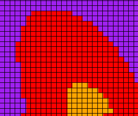
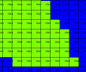
Three differently scaled views of an ArcInfo format elevation grid, showing cell outlines and elevation values.
Most of the raster datasets we will use are single-band, which means that they contain a single "layer" of data. The data can represent elevation, slope, or reflectance (in the case of the black-and-white digital orthophotos we will see later).
These single-band images are viewed with a color mapping, so that the cell value is associated with a particular color. For the orthophotos, the color map is a 256-value greyscale ramp. Other raster data, such as elevation models, can be mapped to color ramps that display elevation ranges, as shown in the image directly above. Most GIF files have a limit of 256 unique values (this is known as 8-bit data, because 2^8 = 256).
Multi-band raster data (such as RGB images or satellite images) are generally displayed with a mixture of red, green, and blue values for each different band in the image.
As you can see, when any of the raster layers are displayed at larger scales, the individual cells become visible. As scale of display increases, precision also decreases, and shapes cannot be precisely represented. All spatial datasets are generalized; however, raster datasets more clearly show their level of generalization. A more complete discussion of generalization in relation to scale is addressed in Scale Issues.
USGS DEMs (Digital Elevation Models) are ASCII (plain text) files which contain georeferencing information as well as point data for elevations on the surface of the earth. Here are the first few lines in the Eatonville, WA 7.5' 30 m DEM:
EATONVILLE, WA 464512215 80000 HAP-81 78-73 08/06/81 BC2 30MX30M INTERVA
EATONVILLE, WA 464512215 FS 1 1 1 10 0.000000000000000D+00
0.000000000000000D+00 0.000000000000000D+00 0.000000000000000D+00
0.000000000000000D+00 0.000000000000000D+00 0.000000000000000D+00
0.000000000000000D+00 0.000000000000000D+00 0.000000000000000D+00
0.000000000000000D+00 0.000000000000000D+00 0.000000000000000D+00
0.000000000000000D+00 0.000000000000000D+00 2 2 4 0.547738572300000D+06
0.517735436400000D+07 0.547628092800000D+06 0.519124459100000D+07
0.557153679500000D+06 0.519132801700000D+07 0.557286257000000D+06
0.517743781300000D+07 0.133000000000000D+03 0.987000000000000D+03
0.000000000000000D+00 10.300000E+020.300000E+020.100000E+01 1 322
1 1 92 1 0.547650000000000D+06 0.518850000000000D+07 0.0
0.170000000000000D+03 0.271000000000000D+03 214 214 215 215 221 227 233
240 246 252 257 261 266 264 262 260 262 263 265 266 266 267 268 269 271
270 269 268 268 268 268 267 265 264 263 262 261 261 261 261 260 259 258
258 258 258 256 254 251 245 239 233 229 225 221 216 212 208 204 200 196
194 192 190 190 190 191 190 190 189 189 188 188 188 188 189 188 187 187
187 186 186 184 183 181 180 179 177 175 173 172 170
1 2 218 1 0.547680000000000D+06 0.518472000000000D+07 0.0
0.133000000000000D+03 0.425000000000000D+03 393 396 400 403 408 414 419
421 423 425 423 422 420 412 403 395 391 386 382 373 365 357 347 338 329
324 318 313 312 312 311 308 305 302 301 300 299 297 295 293 289 285 281
279 277 275 270 265 260 253 247 241 233 226 218 216 213 211 209 207 205
205 205 204 202 200 197 197 197 197 197 197 198 199 200 201 206 211 216
218 219 221 216 211 207 186 166 145 142 138 135 135 135 135 135 135 135
134 134 133 134 135 136 135 135 134 148 163 177 185 192 200 202 203 205
206 208 209 210 212 213 213 213 213 213 214 214 214 214 215 219 224 229
235 241 248 253 258 263 262 261 260 261 263 265 266
266 267 268 269 270 269 268 267 267 267 267 265 264 263 262 261 259 260
260 261 259 257 255 255 255 254 252 250 248 243 238 233 228 224 220 216
212 207 204 200 197 195 193 192 191 191 191 190 190 189 189 188 188 188
188 188 188 187 187 186 186 186 184 183 182 180 179 177 176 174 172 171
...
The first line lists the file name, data input type (HAP = High Altitude Photography), cell size (30MX30M). The subsequent lines list elevations for the lattice mesh points (cell centers).
The DEM file is a data source that is not directly usable in most GIS software, but it can be easily imported into ArcGIS, and used for display and analysis.
Return to top | ahead to Relational Data Model
|
|||||||||||||||
|
The University of Washington Spatial Technology, GIS, and Remote Sensing Page is supported by the School of Forest Resources |
School of Forest Resources |