The alternative harvest systems analysis explores the use of helicopter
yarding and long span yarding as alternatives to conventional harvest systems.
These alternatives are explored in areas where conventional systems would
require the construction of new roads, or the use of existing roads in poor
locations. There are several reasons for performing an analysis of alternative
harvest systems. Most notably, the alternative analysis provides an opportunity
to reduce the impact from roads and perhaps reduce the combined cost of
harvesting and road construction. Additionally, as these undesirable roads
are eliminated, the liabilities from these roads are also eliminated.
Unfortunately, performing an alternative analysis is not as straightforward
as it may seem. The analysis is limited by the technology currently available
for harvest planning. Current software limits the number of options that
can be explored, so it becomes inefficient to provide a complete analysis
of multiple options.
Another difficulty in alternative analysis revolves around the long span
alternative. The setting boundaries for long span harvest systems are, by
nature, different from conventional settings. This becomes a problem when
comparisons are made between the different options. Direct comparisons cannot
be made, so concrete results are difficult to achieve. This problem is compounded
when an alternative analysis is attempted on an individual timber sale rather
than on a landscape wide basis. However, this problem does not exist in
the analysis of helicopter yarding as an alternative because helicopter
settings and conventional settings can be the same.
Although the process of performing an alternative analysis has not yet
reached maturity, by exploring unconventional means of harvesting we hope
to uncover some hidden treasures within the Hoodsport planning area.
Helicopter yarding is an interesting alternative option because it requires
absolutely no new roads. Yarding distances for helicopters are so much larger
than that of conventional systems that there will almost always be a potential
landing on an existing road. However, helicopter systems are typically three
times as expensive as conventional systems. Unless road construction costs
are very expensive, helicopter systems will not be the most cost-effective
option. However, in today’s political and social environment, other factors
such as sediment delivery to streams and road liability must be considered.
This analysis of helicopter yarding as an alternative will look at both
financial considerations and environmental impact. Unfortunately, there
is currently no way to place a monetary value on environmental impact, so
ultimately this remains an upper management decision.
12.2.1 Method
After conventional setting boundaries have been determined, any
setting can be analyzed as a helicopter alternative. However, due
to the high cost of helicopter systems, it only makes sense to analyze
certain types of settings. These are areas that either will provide
relatively little return on the investment of constructing a road
or will cause an excessive amount of damage to the environment. For
instance, if 100 stations of road and two bridge crossings are being
built to access 50 acres of land, it may make more economical sense
to harvest the area with a helicopter system. Even if it did make
economical sense to build the road, the helicopter alternative may
still be better due to the environmental impact of the stream crossings.
So, the first step in an alternative analysis for helicopter yarding
is to make an assessment of the areas that may benefit from a helicopter
system.
The next step is to determine the cost differences between the helicopter
alternative and the conventional systems. It is important to include
the cost of building additional road for the conventional system.
A cost analysis can be performed within the SNAP analysis by including
a helicopter alternative in the analysis. SNAP will then output the
most economical means of harvesting the land.
Next, the environmental impact of the conventional systems must
be weighed against the environmental benefits of using the helicopter
system. These benefits are mostly reduced sediment to streams due
to fewer roads being built.
Finally, these different factors are compared for the conventional
and alternative systems, and the final selection of harvest systems
is made.
12.2.2 Case Studies
Two of the alternatives analyzed in the Hoodsport planning area
present interesting examples of the factors that influence a helicopter
alternative analysis. Case 1 is a situation where a bridge crossing
and several smaller stream crossings are required to access the land.
Case 2 is a situation where there are many existing roads that could
be decommissioned in favor of using a helicopter system.
Case 1: One Bridge Too Many?
Case 1, represented in Figure 48, is a prime example of examining
the tradeoffs between road cost and yarding cost. It also presents
a good example of the environmental impacts of roads. In this situation,
the high cost of road construction due to the bridge crossing and
the other stream crossings suggest that it may be more economical
to avoid building this road. In fact, it is still less expensive to
build the roads and use a conventional harvest system, but the costs
are close enough that it is worth considering the helicopter alternative
for its other benefits.
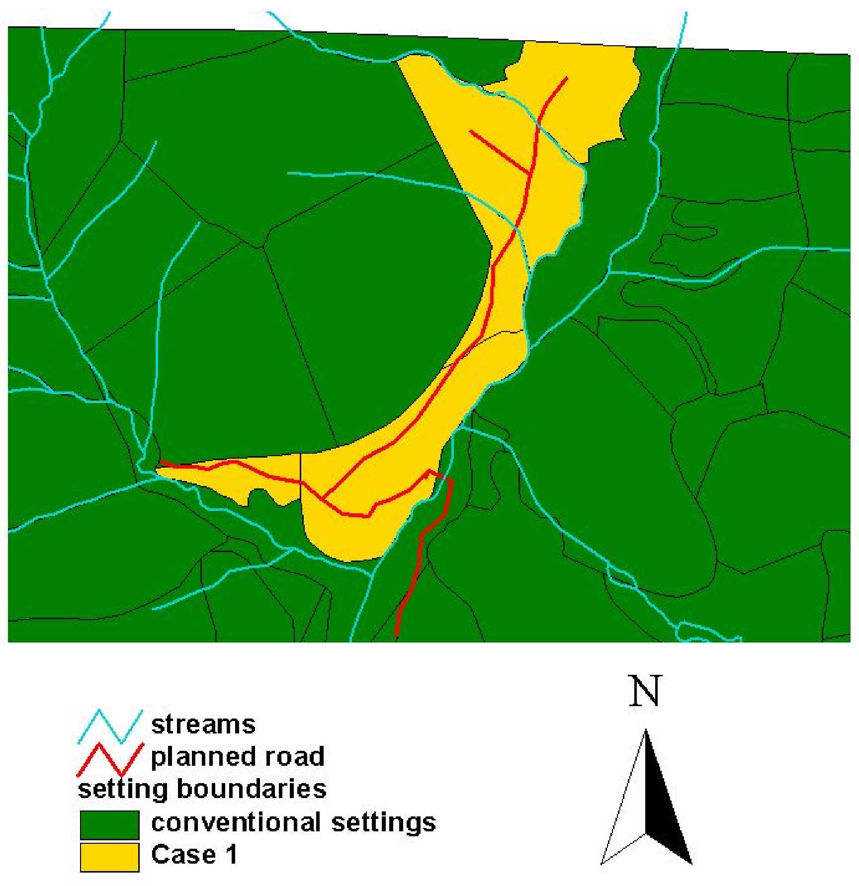
Figure
48. Helicopter Alternative case 1. The planned road will be eliminated
if a helicopter system is used. Otherwise, a bridge will be required
to cross the stream before the road enters the Case 1 settings.
There are several factors that suggest the use of a helicopter system.
The most notable of these is the series of stream crossings required
to access the land. Two type three streams must be crossed here, and
the sediment created by these crossings is a strong encouragement
to avoid building this road.
In addition, adding a road to the land will take a large amount
of land out of timber production. Assuming a right of way width of
50 feet, 100 stations of road corresponds to about 12 acres of lost
timber production land. In this situation, that is almost 10% of the
available land. With this factored in, the helicopter alternative
becomes a viable option.
However, this becomes even more complicated when the possibility
of using temporary roads is factored in. Table 14 provides a summary
of some potential harvest options.
Table
14 Potential harvest options to be used in Case 1.
|
Road Type
|
Harvest Type
|
Sediment
|
Cost
|
|
Temporary Summer
|
Conventional
|
Low
|
Low
|
|
Temporary Winter
|
Conventional
|
High
|
Low
|
|
Permanent
|
Conventional
|
High
|
Low
|
|
None
|
Helicopter
|
Low
|
High
|
From Table 14, you can see that building a temporary road and harvesting
in the summer is the best option. However, since this land is low
in elevation, it has good potential for winter harvest. If harvesting
in the winter is opted for, the tradeoffs here make for a very difficult
decision. How much is sediment really worth? At this time, there is
no answer to this question. It must be decided on a case by case basis,
depending on the political, social, and environmental conditions of
the area. The important thing here is to see that there are several
options, and they must all be considered when making a decision.
Case 2: Too Many Roads vs. Helicopter
Case 2 examines a very different scenario than case 1. Case 2 examines
an area with an excessive number of existing roads (See Figure 49).
The tradeoff here is between keeping the roads and using a conventional
harvest system or decommissioning the existing roads and using a helicopter
system. Clearly the conventional system would cost less money since
the roads have already been built. The real question here revolves
around the environmental impact of the existing roads. How much impact
do these roads have on the environment, and does this impact justify
the added cost of using a helicopter system?
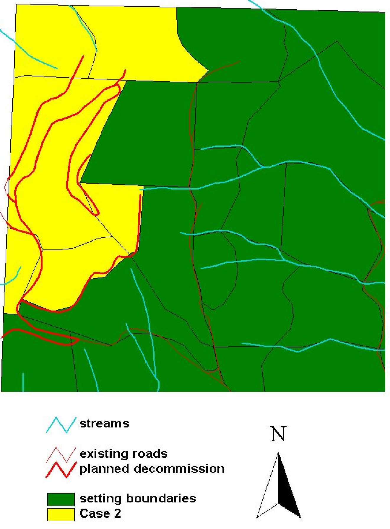
Figure
49. The thick red lines represent roads that would be decommissioned
if the Case 2 settings were selected for helicopter systems rather
than the conventional systems. Notice that there are no stream crossings
in the roads to be decommissioned, so the environmental impact of
the existing roads is minimal.
In this case, despite the 100 stations of road used to access only
71 acres of timber, the answer is that the existing roads have little
environmental impact, and so the cost of decommissioning the roads
and using a helicopter system can not be justified. As you can see
in Figure 49, although there are many roads in a small area, there
are no stream crossings. Therefore, the impact of these roads on sedimentation
is very low. The only remaining questions are whether the liability
of keeping the existing roads outweighs the economic benefits of keeping
them open, and how much of an impact the lost production ground has
on the situation. Based on the same logic from case 1, approximately
12 acres of land is lost from timber production. That is 17% of the
available land! However, it is still more economical in this case
to use the conventional alternative.
12.2.3 Results
Five major areas were examined in the helicopter alternative analysis.
The location of these areas can be seen in Figure 50. The results
from the helicopter alternative analysis are shown in Table 15.
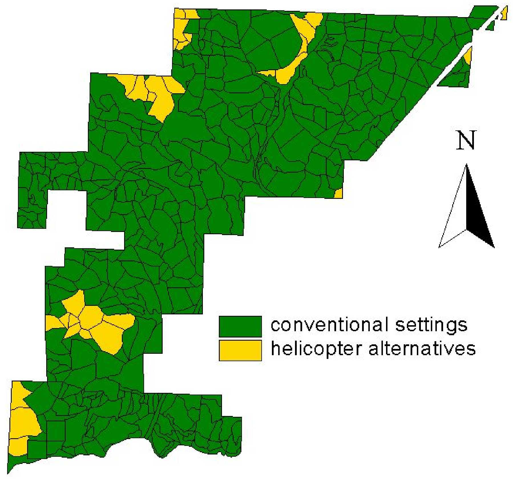
Figure
50. Helicopter alternative settings are highlighted in yellow.
Notice the five distinct groups that have been analyzed in detail.
Groups are labeled counterclockwise from the top down heli1 through
heli5.
Table
15. Summary of results from the helicopter yarding alternative
analysis.
|
|
Heli 1
|
Heli 2
|
Heli 3
|
Heli 4
|
Heli 5
|
|
Acres accessed
|
122
|
71
|
186
|
276
|
159
|
|
Road Eliminated (Sta.)
|
102+62
|
100+86
|
91+02
|
106+65
|
82+68
|
|
Sediment Eliminated tons/year
|
19
|
.08
|
9
|
.23
|
4.37
|
|
Harvest cost of helicopter alternative
|
620,610
|
606,078
|
923,700
|
1,039,825
|
1,912,781
|
|
Conventional harvest cost plus road costs
|
485,020
|
224,169
|
669,996
|
732,315
|
1,450,781
|
Overall, it is clear that helicopter yarding is typically more expensive
than conventional systems. However, when other factors such as sedimentation
caused by roads are factored in, the potential benefits of using a
helicopter system start to make a strong argument. Therefore, the
decision to utilize helicopter systems as an alternative must continue
to be made on a case by case basis, looking at the various benefits
for each system before a final decision can be made.
As part of the alternative yarding analysis, the next alternative to be
looked at is long span yarding. The purpose of long span yarding is to minimize
sediment delivery to streams and reduce the construction of unnecessary
roads. Within the Hoodsport DNR block, there were ten timber units that
qualified as possible sites for long span yarding. These areas were chosen
due to good deflection over existing streams and they all were able to prevent
the construction of planned roads that pertained to conventional yarding
units (see Figure 51).
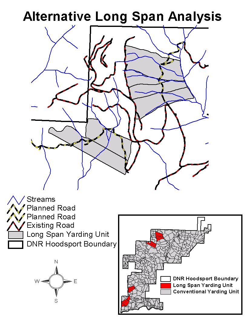
Figure
51 Alternative Long Span Analysis areas within the Hoodsport DNR block.
The alternative analysis area within the Hoodsport DNR block that will
be considered for further analysis is the expanded area shown in Figure
51. This area is accessed via forest service road 2572 and borders the Five
Flags timber sale boundary. The reason why this area was chosen for analysis
was because the Five Flags timber sale was laid out based on stream buffers.
If the Five Flags timber sale were laid out based on yarding capabilities,
it can be seen that yarding distances of 3000 – 4000 feet can be achieved
versus the conventional distances of 1200 – 2000 feet. Further more, the
planned construction of a road accessing the Five Flags timber sale area
can be prevented. Note, summary statistics will be shown in the following
sections for all ten of the long span units, but all examples will pertain
to the Five Flags timber sale area.
The analysis of alternative long span yarding will look at three possible
long span scenarios, the cost yarding with long span, a comparison between
conventional and long span yarding, and then will summarize with the results.
12.3.1 Alternative Long Span Scenarios
As part of the long span analysis, three possible situations can
be modeled for further analysis. The three possible situations are
hanging to the edge of a Riparian Management Zone (RMZ), hanging across
a RMZ and yarding to edge of RMZ, and yarding over an RMZ with full
deflection. All three situations were looked at using a 90-foot tower
live skyline system. It should be noted that the live skyline analysis
performed by LoggerPC may slightly overestimate conditions since it
assumes a perfect operator who continually adjusts the skyline length
to maximize payload.
Figure 52 shows an example of the first scenario, hanging to the
edge of a RMZ.
Figure
52 Hanging to the edge of a RMZ with partial suspension.
Figure 52 has an external yarding distance (EYD) of 2,400 feet and
a limiting payload of 9,363 lbs. at turning point 33 and a tailhold
of 50 feet. For the record, this same profile was evaluated with full
suspension and had a limiting payload of 917 lbs. at turning point
33 (See Figure 53).
Figure
53 Hanging to the edge of a RMZ with full suspension.
The second long span scenario that can be evaluated is hanging across
a RMZ and yarding to the edge of the RMZ. For this situation, the
EYD was 4,000 feet with a limiting payload of 14,081 at turning point
48. This example shows that by having a 50-foot tailhold across the
RMZ makes it possible to have full suspension, where it was not possible
in the first situation (See Figure 54).
Figure
54 Hanging across a RMZ and yarding to the edge of the RMZ.
The third long span scenario is yarding over an RMZ with full deflection.
This scenario had an EYD of 3600 feet and a limiting payload of 3,199
lbs. at turning point 68 with a tailhold height of 2-feet. This profile
was taken from unit 5, which is Southwest of the Five Flags timber
sale (See Figure 55 and refer back to Figure 51).
Figure
55 Yarding over an RMZ with full deflection.
12.3.2 Hoodsport Long Span Statistics
As previously stated, there are ten possible long span units within
the Hoodsport DNR block. Due to the limiting capabilities of SNAP,
long span analysis has to be done manually and then compared to the
SNAP results for conventional yarding systems. For reference, the
ten long span units are numbered in ascending order going from South
to North (See Figure 51).
From the data provided (GIS layers), the following information was
gathered for the ten long span units (See Table 16).
Table
16 Long Span analysis data.
|
Unit No.
|
Landing ID
|
EYD
|
LYD
|
AYD
|
Area (Acres)
|
Bf/log
|
Mbf/acre
|
|
1
|
4-LS-7
|
1850
|
150
|
925
|
16.53
|
48.27
|
13.93
|
|
|
4-LS-13
|
2250
|
150
|
1125
|
19.38
|
48.27
|
13.93
|
|
|
4-LS-14
|
2250
|
150
|
1125
|
20.20
|
48.27
|
13.93
|
|
|
4-LS-15
|
2050
|
150
|
1025
|
12.95
|
48.27
|
13.93
|
|
2
|
4-LS-12
|
2650
|
150
|
1325
|
22.13
|
46.75
|
14.51
|
|
|
4-LS-16
|
2250
|
150
|
1125
|
20.57
|
46.75
|
14.51
|
|
3
|
4-LS-17
|
1750
|
150
|
875
|
16.53
|
46.25
|
11.67
|
|
|
4-LS-18
|
1400
|
150
|
700
|
12.21
|
45.42
|
12.25
|
|
|
4-LS-19
|
1100
|
150
|
550
|
11.29
|
44.59
|
12.83
|
|
4
|
4-LS-3
|
2450
|
150
|
1225
|
21.95
|
80.89
|
18.67
|
|
|
4-LS-5
|
2700
|
150
|
1350
|
20.20
|
82.77
|
17.78
|
|
|
4-LS-6
|
2600
|
150
|
1300
|
18.27
|
74.41
|
17.06
|
|
5
|
4-LS-1
|
2350
|
150
|
1175
|
25.71
|
73.68
|
15.26
|
|
|
4-LS-4
|
2350
|
150
|
1175
|
18.37
|
67.62
|
13.59
|
|
6
|
2-RT-8
|
3400
|
150
|
1700
|
30.95
|
63.59
|
19.46
|
|
|
2-LS-9
|
4000
|
150
|
2000
|
37.19
|
63.96
|
19.59
|
|
7
|
2-LT-6
|
2450
|
150
|
1225
|
28.65
|
62.83
|
19.20
|
|
|
2-LT-7
|
2300
|
150
|
1150
|
22.22
|
62.83
|
19.20
|
|
8
|
2-LS-4
|
2650
|
150
|
1325
|
20.66
|
114.98
|
23.49
|
|
|
2-RT-5
|
2700
|
150
|
1350
|
25.07
|
114.98
|
23.49
|
|
9
|
2-LT-3
|
2700
|
150
|
1350
|
32.87
|
114.98
|
22.44
|
|
10
|
2-LS-1
|
2650
|
150
|
1325
|
29.29
|
160.97
|
22.44
|
|
|
2-LS-2
|
2750
|
150
|
1375
|
41.51
|
102.65
|
22.44
|
From Table 16, summary statistics were calculated for future input
into the Binkley Production Equation, which will be discussed in section
12.3.3. Table 17 shows the averages computed for the ten long span
units.
Table
17 Long span unit averages computed for Binkley production equation.
|
Unit No.
|
No. corridors
|
AYD
|
Area (Acres)
|
Bf/log
|
Mbf/acre
|
Slope Under Cable (%)
|
Slope Perp. Cable (%)
|
|
1
|
4
|
1050.0
|
69.05
|
48.27
|
13.93
|
39.0
|
28.8
|
|
2
|
2
|
1225.0
|
42.70
|
46.75
|
14.51
|
42.0
|
15.0
|
|
3
|
3
|
708.0
|
40.04
|
45.42
|
12.25
|
50.0
|
30.0
|
|
4
|
3
|
1292.0
|
60.42
|
79.35
|
17.84
|
63.0
|
33.3
|
|
5
|
2
|
1175.0
|
44.08
|
70.65
|
14.43
|
75.0
|
47.0
|
|
6
|
2
|
1850.0
|
68.14
|
63.77
|
19.53
|
32.5
|
17.5
|
|
7
|
2
|
1187.5
|
50.87
|
62.83
|
19.20
|
37.5
|
15.0
|
|
8
|
2
|
1337.5
|
45.73
|
114.98
|
23.49
|
35.5
|
10.0
|
|
9
|
1
|
1350.0
|
32.87
|
114.98
|
22.44
|
37.0
|
15.0
|
|
10
|
2
|
1350.0
|
70.80
|
131.81
|
22.44
|
34.5
|
12.5
|
The results of Table 17 show that for some of the long span units,
Mbf per acre is relatively low. This becomes a serious problem with
regards to the Binkley production equation, which will be further
explained in section 12.3.3.
12.3.3 Alternative Long Span Cost Analysis
In order to perform a long span cost analysis, the amount of planned
road for conventional yarding that overlaps with the long span units
has to be determined. Along with the amount of road that will not
have to be built, costs have to be analyzed for constructing, actively
maintaining, inactivating, and abandoning these roads over the next
60 years so that a comparison between conventional and long span yarding
can be made.
The first step in performing this cost analysis is to input the
information displayed in Table 17 into the Binkley production equation
plus the additional information shown in Table 18.
Table
18 Input data for Binkley production equation
|
Unit No.
|
No. corridors
|
Int. Support
|
Logs/Turn
|
Crew No.
|
% Prod. Time
|
Hours/day
|
O&O Costs
|
Rig.
Costs
|
Rd. Costs
|
|
1
|
4
|
0
|
4.5
|
5
|
90
|
8
|
$333
|
$333
|
$0.00
|
|
2
|
2
|
0
|
4.5
|
5
|
90
|
8
|
$333
|
$333
|
$0.00
|
|
3
|
3
|
0
|
4.5
|
5
|
90
|
8
|
$333
|
$333
|
$0.00
|
|
4
|
3
|
0
|
4.5
|
5
|
90
|
8
|
$333
|
$333
|
$0.00
|
|
5
|
2
|
0
|
4.5
|
5
|
90
|
8
|
$333
|
$333
|
$0.00
|
|
6
|
2
|
0
|
4.5
|
5
|
90
|
8
|
$333
|
$333
|
$0.00
|
|
7
|
2
|
0
|
4.5
|
5
|
90
|
8
|
$333
|
$333
|
$0.00
|
|
8
|
2
|
0
|
4.5
|
5
|
90
|
8
|
$333
|
$333
|
$0.00
|
|
9
|
1
|
0
|
4.5
|
5
|
90
|
8
|
$333
|
$333
|
$0.00
|
|
10
|
2
|
0
|
4.5
|
5
|
90
|
8
|
$333
|
$333
|
$0.00
|
After inputting the data from Table 17 and Table 18 into the Binkley
equation, the following results were obtained.
Table 19 Results of Binkley
production equation
|
Unit No.
|
$/Mbf
|
Total Yarding Cost ($)
|
|
1
|
468.94
|
451 083.18
|
|
2
|
328.41
|
203 473.16
|
|
3
|
365.55
|
179 283.27
|
|
4
|
351.58
|
378 908.33
|
|
5
|
789.83
|
502 181.93
|
|
6
|
270.43
|
359 766.08
|
|
7
|
245.45
|
239 742.17
|
|
8
|
128.99
|
138 560.29
|
|
9
|
141.80
|
104 605.02
|
|
10
|
119.71
|
190 185.79
|
The next step is to calculate the amount of planned road that will
not be built due to long span yarding. For this, the long span units
had to be merged into long span areas due to planned road segments
that were laid out through multiple long span units. Table 20 shows
the amount of unnecessary road associated with each long span area.
Table
20 Number of road stationing associated with each long span area.
|
Area No.
|
Unit No.
|
Unnecessary Road (STA)
|
|
1
|
1
|
|
|
|
2
|
|
|
|
3
|
|
|
|
|
68
|
|
2
|
4
|
|
|
|
5
|
|
|
|
|
8
|
|
3
|
6
|
|
|
|
7
|
|
|
|
|
78
|
|
4
|
8
|
|
|
|
9
|
|
|
|
10
|
|
|
|
|
44
|
Before going onto further cost analysis, roads cost estimates were
obtained from the DNR for High, Medium, and Low road classes. For
this analysis, a road class of medium was chosen to best model the
planned roads. Table 21 shows cost estimates as pertaining to the
Hoodsport DNR block.
Table
21 DNR road cost estimates for the Hoodsport block
|
Cost
|
$/STA
|
Occurrence
|
|
Construction
|
1 850
|
One time
|
|
Reconstruction
|
275
|
One time
|
|
Inactivation
|
26
|
One time
|
|
Abandonment
|
90
|
One time
|
|
Active Maintenance
|
17
|
Annual
|
|
Inactive Maintenance
|
8
|
Annual
|
Now, with the information provided in Table 21, a cost of dollars/station
and total road construction costs saved can be computed as Net Present
Value (NPV) over a 60-year period with an interest rate of 6 percent.
The Net Present Value for these costs is displayed in Table 22. Note
that these costs are the amount saved by not building these roads
due to long span yarding.
Table
22 Comparison of Active, Inactive, and Abandonment NPV costs.
|
Area No.
|
Unnecessary Road (STA)
|
Active (NPV)
|
Inactive (NPV)
|
Abandon (NPV)
|
|
|
|
$/STA
|
$ Total
|
$/STA
|
$ Total
|
$/STA
|
$ Total
|
|
1
|
68
|
2 124.74
|
144 482.58
|
2 111.51
|
143 582.39
|
2 155.73
|
146 589.34
|
|
2
|
8
|
2 124.74
|
16 997.95
|
2 111.51
|
16 892.05
|
2 155.73
|
17 245.80
|
|
3
|
78
|
2 124.74
|
165 730.02
|
2 111.51
|
164 697.45
|
2 155.73
|
168 146.60
|
|
4
|
44
|
2 124.74
|
93 488.73
|
2 111.51
|
92 906.25
|
2 155.73
|
94 851.93
|
12.3.4 Economic comparison of Long Span
and Conventional Yarding
After receiving the results from SNAP for conventional yarding,
these costs had to be compared to long span yarding costs. Before
doing this, the percentage of each conventional unit that was in a
long span unit had to be determined. The conventional yarding costs
were then weighted and averaged in order to compare the cost of yarding
a long span unit to a conventional. This averaging was required because
conventional sale boundaries do not match up identically with long
span boundaries. Table 23 shows the results of the comparison between
long span and conventional yarding costs for the four long span areas
within the Hoodsport block.
Table
23 Economic comparison of Long Span and Conventional Yarding.
|
Area No.
|
Long Span ($/Mbf)
|
Conventional ($/Mbf)
|
Difference ($/Mbf)
|
|
1
|
323
|
260
|
63
|
|
2
|
236
|
179
|
57
|
|
3
|
260
|
192
|
68
|
|
4
|
127
|
108
|
19
|
In Table 23, it can be seen that the cost to long span yard is greater
in all four areas than the cost to yard conventionally. The reason
for this is due to the low timber volumes within these four areas.
Although it is not economically feasible to long span these four areas
currently, it may be 10 to 15 years in the future. The reason for
this is that long span yarding is heavily dependent on large volumes
of timber, which translates into large turn weights.
Current DNR policy encourages alternative analysis, specifically the use
of long span yarding systems, as a way to reduce road length. The goal of
reducing road length/density, is the reduction of sediment input into the
stream system. After trying to compare long span results to conventional
yarding results, it became apparent that we were comparing two different
things. Below we will discuss the problems we found with direct comparison
of conventional and alternative yarding systems, and some solutions to this
problem.
12.4.1 Setting Boundaries
Due to the differences between long span and conventional system
requirements and their associated production costs, the resultant
setting boundaries for long span units end up being very different
from the shape of conventional setting boundaries. In the long span
case settings tend to be a single, long, narrow corridor approximately
4000 feet long by 300 feet wide. Conventional settings on the other
hand tend to be circular or semi-circular and radiate outward from
a central landing for a distance of no more than 2000 feet. Therefore,
due to the differences in setting shapes it only makes sense to compare
alternative yarding systems to conventional systems at the watershed
or landscape level and not at the individual sale level.
With the exception of ground units, it is infeasible to use the
same setting boundaries for conventional and alternative analysis.
Due to topographic and mechanical restrictions associated with long
span yarding, long span settings are rarely, if ever, the same as
conventional settings. Therefore, long span analysis should only be
attempted on a landscape wide management plan. On the other hand,
alternative analysis will work at the timber sale level, so long as
ground systems are compared to ground systems and/or conventional
cable systems to helicopter systems.
12.4.2 Current Technology
Scheduling and Networking Analysis Program (SNAP) can pick between
conventional and helicopter alternatives. This is because they share
setting boundaries. Where SNAP runs into problems is in the comparison
between long span and conventional analysis. The software is unable
to pick between long span and conventional because if it picks long
span in one area, it must readjust the setting boundaries of the adjacent
settings. Figure 56 shows the relationship between conventional and
long span setting boundary shapes.
Figure
56. Comparing long span and conventional setting boundaries.
As shown in Figure 56, each long span yarding unit includes multiple
conventional yarding units.
Using the current version of SNAP there are only two ways that we
can compare long span settings to conventional settings. The first
is to create two separate setting boundary maps, one with conventional
and helicopter settings, and one with long span, helicopter, and conventional
settings. Once the two layers have been completed, they must be run
through the software separately and compared manually. The problem
with this method is by only allowing all long span or no long span,
there is no way to only select the best long span settings and keep
all other conventional settings.
The second method is to create one setting boundary map with the
harvest system (long span, helicopter, or conventional) fixed. This
method removes SNAP’s ability to pick the harvest system with the
lowest costs. The problem here is that the output of this method is
only the scheduling and harvest costs, whereas in the first method
the output is harvest system, scheduling, and harvest costs.
12.4.3 Future Technology
Currently, this process requires so many iterations that it becomes
infeasible to do by hand. Therefore, the most efficient way to complete
this analysis will be to update the current software to include a
flowchart it can follow as it makes decisions in the planning process.
For example, if long span is selected for one area, the associated
road will be removed and no landings can be located on it. Then any
areas accessed by that road must be yarded by one of two options,
helicopter or long span.
This technology will require a more interactive user interface that
will put control back into the hands of the planner. By prompting
the planner at major decision points, the software can take advantage
of both the planner’s experience with long span harvest planning,
and the speed of today’s computer processors.