13 Harvest Scheduling
13.1 Introduction
This chapter will discuss the inputs and outputs of the SNAP program and
how SNAP was used to schedule road construction and create a harvest plan
for the North Hoodsport planning area. The SNAP program uses information
from two GIS coverages and growth data provided by DNR to determine when
roads should be constructed as well as when harvest units should be put
up for bid. SNAP then attempts to maximize the value of wood at the mill
my minimizing road construction, harvest, and haul costs.
13.2 SNAP Inputs
SNAP uses two GIS coverages to analyze an area: a polygon coverage of the
harvest settings, and a line coverage of the proposed road network. The
polygon coverage was digitized into ArcInfo based on probable landing locations
and reasonable external yarding distances. Into each of these setting polygons,
21 attributes were added:
- AREA The harvestable acreage of the polygon
- ENT1 The road node ID where timber will be harvested to for #1
- ENT2 The road node ID where timber will be harvested to for #2
- ENT3 The road node ID where timber will be harvested to for #3
- SIL1 Candidate silvicultural treatment #1
- SIL2 Candidate silvicultural treatment #2
- SIL3 Candidate silvicultural treatment #3
- STAT Used to hardwire a unit into a specific harvest period
- SPE1 Used to identify different species -- we used only Douglas Fir
- VOL1 Volume per acre of SPE1 in MBF
- SERS The current seral stage of the unit
- HAR1 Candidate harvest method #1 for the unit
- HAR2 Candidate harvest method #2 for the unit
- HAR3 Candidate harvest method #3 for the unit
- AYD1 Average Yarding Distance #1
- AYD2 Average Yarding Distance #2
- AYD3 Average Yarding Distance #3
- HVC1 Harvest Cost $/MBF Gross #1
- HVC2 Harvest Cost $/MBF Gross #2
- HVC3 Harvest Cost $/MBF Gross #3
- ATO1 An optional attribute used for adjacency
The road coverage was digitized onto the existing DNR TRANS coverage. The
proposed roads were digitized from base maps, field maps, and survey notes,
where possible. For each road arc, three attributes were added:
RDST The status of the road, existing, reconstruct, or new construction
MACL Maintenance class
FXOR Used to tell SNAP a fixed override cost for road construction
In addition to these factors, some variables were input directly into SNAP,
including the average speed on the road.
13.3 Growth Rates
SNAP models the ways in which stand volumes change over time based on a
series of decision trees. The decision trees contain average annual growth
rates for each scheduling period based on the age and operational history
of each stand. SNAP has the option of performing certain user-specified
silvicultural treatments based on the seral stage of each stand (the term
seral stage is somewhat of a misnomer here as it refers to the age and operational
history of a stand rather than its structure).
Stands that are never treated will increase in volume at the user-specified
passive rate. When a silvicultural treatment is performed, the appropriate
volume is removed from the stand inventory and the stand continues to grow
along a new branch of the decision tree.
For example, in the following sample table (Table 24), SNAP may choose
to do nothing or to perform a pre-commercial thin at seral stage "10-14".
If no operation is performed, the stand volume will continue along the passive-rate
branch, moving on to seral stage "15-19" and increasing at a rate
of 7% in that period. If a pre-commercial thin is performed, 30% of the
volume will be removed and the stand will thereafter grow along the PCT-rate
branch. It will move on to seral stage "15-19 PCT," increasing
at a rate of 11% in that period. This example is purely hypothetical, because
pre-commercial thinning was not an option in the Hoodsport planning area.
SNAP has the option of performing other operations such as commercial thins
and clearcuts in later seral stages. Clearcuts reset stands to the initial
seral stage "0-4".
Table 24.
Sample SNAP Growth Rate Decision Tree. Follow Passive Rate, CT Rate, and
PCT Rate down the column until treatments indicate otherwise.
|
Seral Stage
|
Possible Treatments
|
Volume Removed
|
Passive Rate
|
CT Rate
|
PCT Rate
|
Next Stage
|
|
0-4
|
None
|
None
|
60%
|
|
|
5-9
|
|
5-9
|
None
|
None
|
20%
|
|
|
10-14
|
|
10-14
|
None, PCT
|
None, 30%
|
9% ---------
|
---------à
|
11%
|
15-19, 15-19 PCT
|
|
15-19
|
None, PCT
|
None, 30%
|
7% ---------
|
---------à
|
10%
|
20-24, 20-24 PCT
|
|
20-24
|
None, PCT, CT
|
None, 30%, 40%
|
6% ------à
|
9%
|
ß -----8%
|
25-29, 25-29 CT, 25-29 PCT
|
|
25-29
|
None, CT
|
None, 40%
|
5% ------à
|
8%
|
ß -----7%
|
30-34, 30-34 CT, 30-34 PCT
|
|
30-34
|
None, CT
|
None, 40%
|
4.5%----à
|
7%
|
ß -----6%
|
35-39, 35-39 CT, 35-39 PCT
|
13.3.1 Sources of Growth Rates
Growth rates were provided directly from DNR. More information on
growth rates is located in chapter 6.
13.3.2 Limitations of SNAP Growth Modeling
The accuracy of SNAP’s modeling of changes in landscape volume over
time is limited both by the quality of the initial data and by the
low degree of growth rate variability SNAP can recognize within a
landscape.
Chapter 6 discusses the likely errors in the estimates of initial
volumes and future growth rates in some detail. In general, the initial
volume values may be reflective of actual landscape conditions while
the growth rates are likely optimistic.
The degree to which SNAP can recognize inter-stand variation in
growth is limited by the number and level of detail of the decision
trees it is given to work with. Each additional decision tree requires
a new set of growth rates for each possible operational decision.
Every time the number of decision trees is doubled the scheduling
optimization process becomes as much as four times longer and more
complex. In practice, landscape variation is limited to the variation
of the initial volumes. Thereafter, every stand of the same age and
operational history grows the same way.
13.4 Cost and Revenue Inputs
Cost inputs into SNAP include road construction, harvest, and haul costs.
Revenue is determined at the Mill.
13.4.1 Road Construction and Harvest Costs
Road construction costs were hard-wired into the transportation
coverage attributes. The method for determining these costs is discussed
in chapter 11. Harvest costs were based on the production equations
discussed in chapter 7. These costs were hard-wired into the settings
coverage attributes.
13.4.2 Haul Costs
The haul costs were input directly into SNAP. Haul costing is done
using the average MBF load per truck and the average cost of trucking
per mile. For the Hoodsport area, we assumed $1.00 per minute for
hauling with a load of 4.5 MBF. Road maintenance costs are also calculated
as part of the haul cost. We assumed $1.33 /MBF/Mile for all roads.
13.4.3 Mill Revenue
Revenues are generated at the mill. We specified one mill in Shelton
that currently pays $500.00 per MBF for Douglas Fir. This mill price
is appreciated over time at 3%, while costs increase at a rate of
1%. Multiple mills can be designated in SNAP, but we used just one
for comparison purposes.
13.5 Harvestable Area
The STAT attribute in the settings coverage tells SNAP whether each polygon
is harvestable or not. In Figure 57, light blue polygons are not harvestable.
All other polygons are harvestable according to their varying restrictions.
These no-harvest zones include riparian buffers, rock outcrops, and other
types of leave areas. Some wetland buffers are included, but these are not
all inclusive.
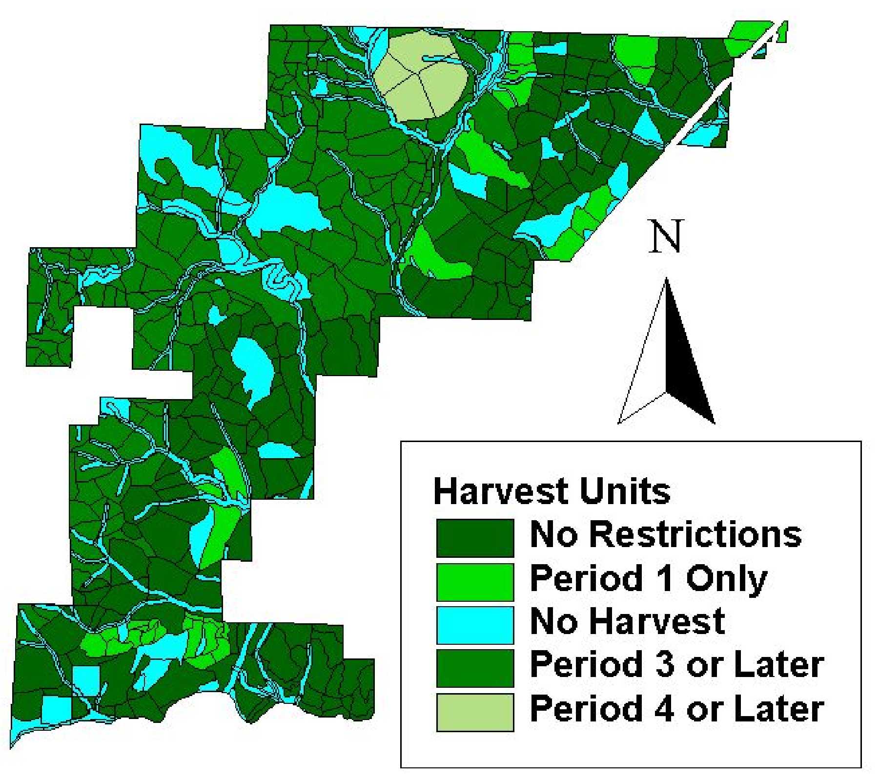
Figure
57. No Harvest areas are indicated in light blue. These areas include
riparian buffers, rock outcrops, and various other no harvest units.
13.6 Habitat Considerations
There are three spotted owl circles that impact the North Hoodsport planning
area. The settings that are affected by these circles are displayed in Figure
58. Management in these areas was delayed for 10 years, bringing us through
period 2. These settings were opened for management in period 3.
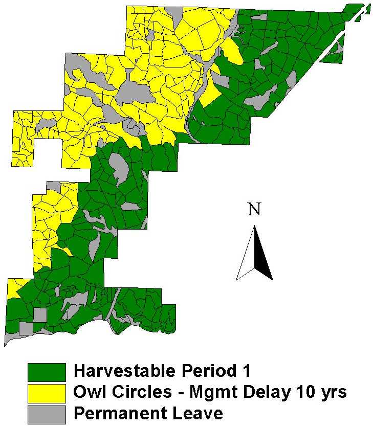
Figure
58. Three owl circles impact the North Hoodsport planning area. Settings
affected by these owl circles were set on a management delay of 10 years.
13.7 DNR Five Year Action Plan
DNR provided a five year action plan to be incorporated into the SNAP analysis
(See Figure 59). Except for the three sales affected by the owl circles,
each of DNR’s planned sales was hard-wired to be harvested during the first
period. It is interesting to note that the DNR planned sales actually return
a higher net present worth than an unrestricted SNAP analysis returns. However,
this is due to the fact that the DNR action plan harvests more than the
15,000 MBF set as a goal for period 1.
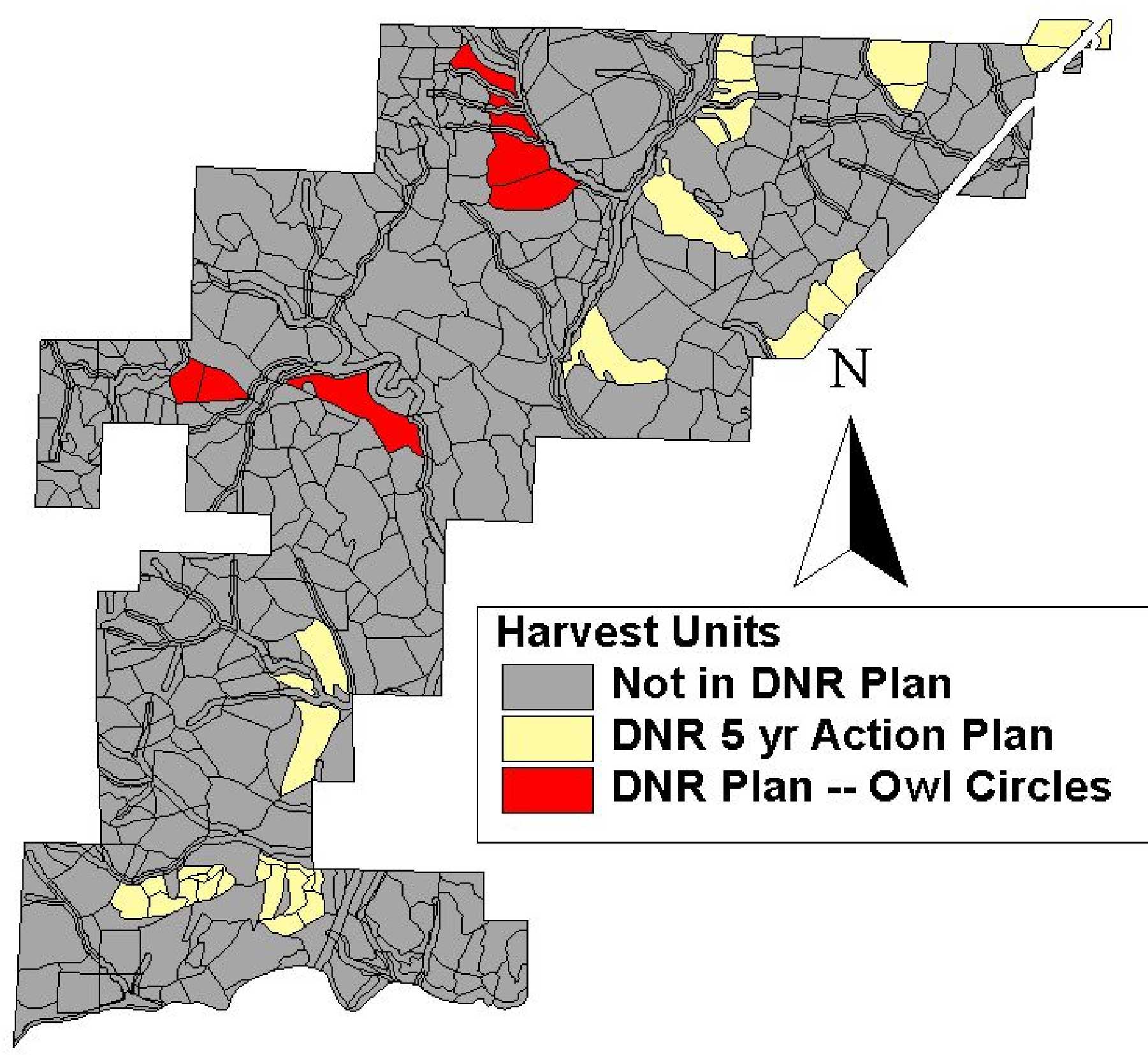
Figure
59. The five-year action plan provided by DNR. Yellow sales were hard-wired
for harvest in period 1. Pink units were within the owl circles, so harvest
was not allowed for the first two periods.
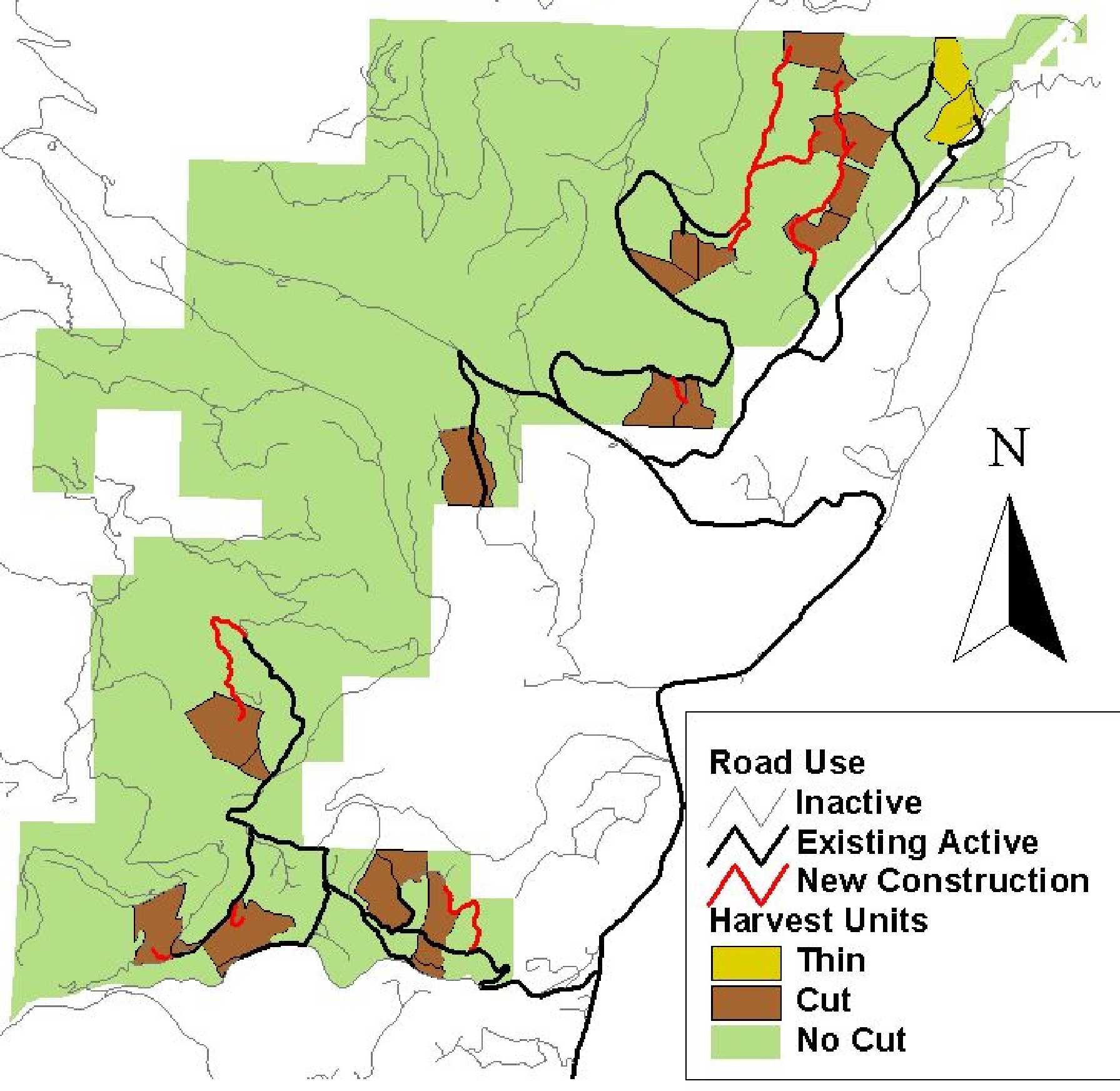
13.8 Harvest and Transportation Schedule
The following five maps show the landscape at five year intervals over
the next 25 years. Each map shows the roads that are constructed during
that time period as well as the specific harvest units that are put up for
sale. To comply with the HCP and FPA, adjacency and maximum harvest acreage
constraints were set. The maximum adjacent harvest area was set at 100 acres,
according to the HCP requirements. Based on the FPA, adjacency was defined
as units younger than 5 years that share more than 200 feet of common boundary.
13.8.1 Period 1: 1999-2004
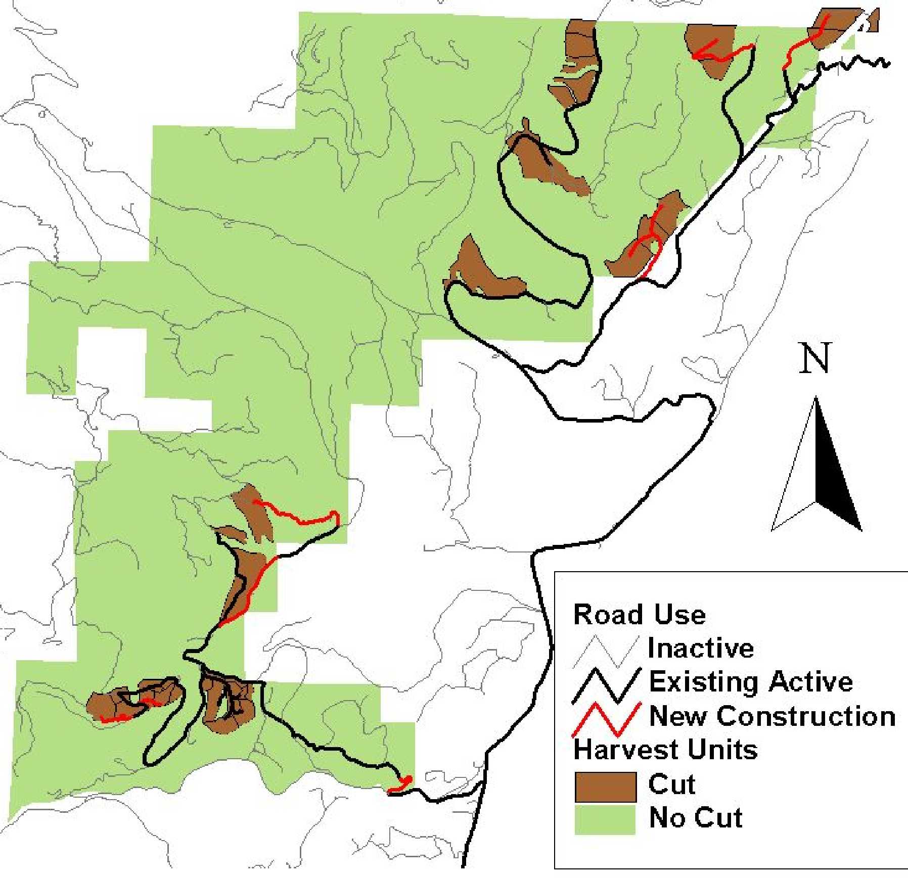
Figure
60. Road and harvest schedule based on SNAP analysis, 1999-2004.
The settings harvested in period 1 (Figure 60) consist of the units
identified in DNR’s five-year action plan. The western half of the
planning area could not be harvested in this period due to the existence
of three owl circles. Three planned DNR sales were lost due to the
owl circles, but the remaining sales easily reach the 15,000 MBF goal
for period 1. A total of 20,731 MBF was harvested during this period.
This volume may change depending upon the status of the North Beacon
sale in the northeast corner of the planning area. The sale was included
in this analysis.
Roads of interest in this period include the Jorsted Bypass and
the Shirt Pocket Road. The Jorsted Bypass provides an alternative
to rebuilding the slide-destroyed Jorsted Road. The Shirt Pocket Road
provides an alternative to the washed out bridge near the detached
sale. More information on these roads can be found in the Hoodsport
Transportation Systems Report. A summary of period 1 activity is located
in Table 25.
Table
25. Summary of period 1 road and harvest activities.
|
Managed Area
|
Harvest Volume
|
Existing Roads
|
New Construction
|
Revenue
|
|
730 acres
|
20731 MBF
|
16.3 miles
|
4.6 miles
|
$8.34 million
|
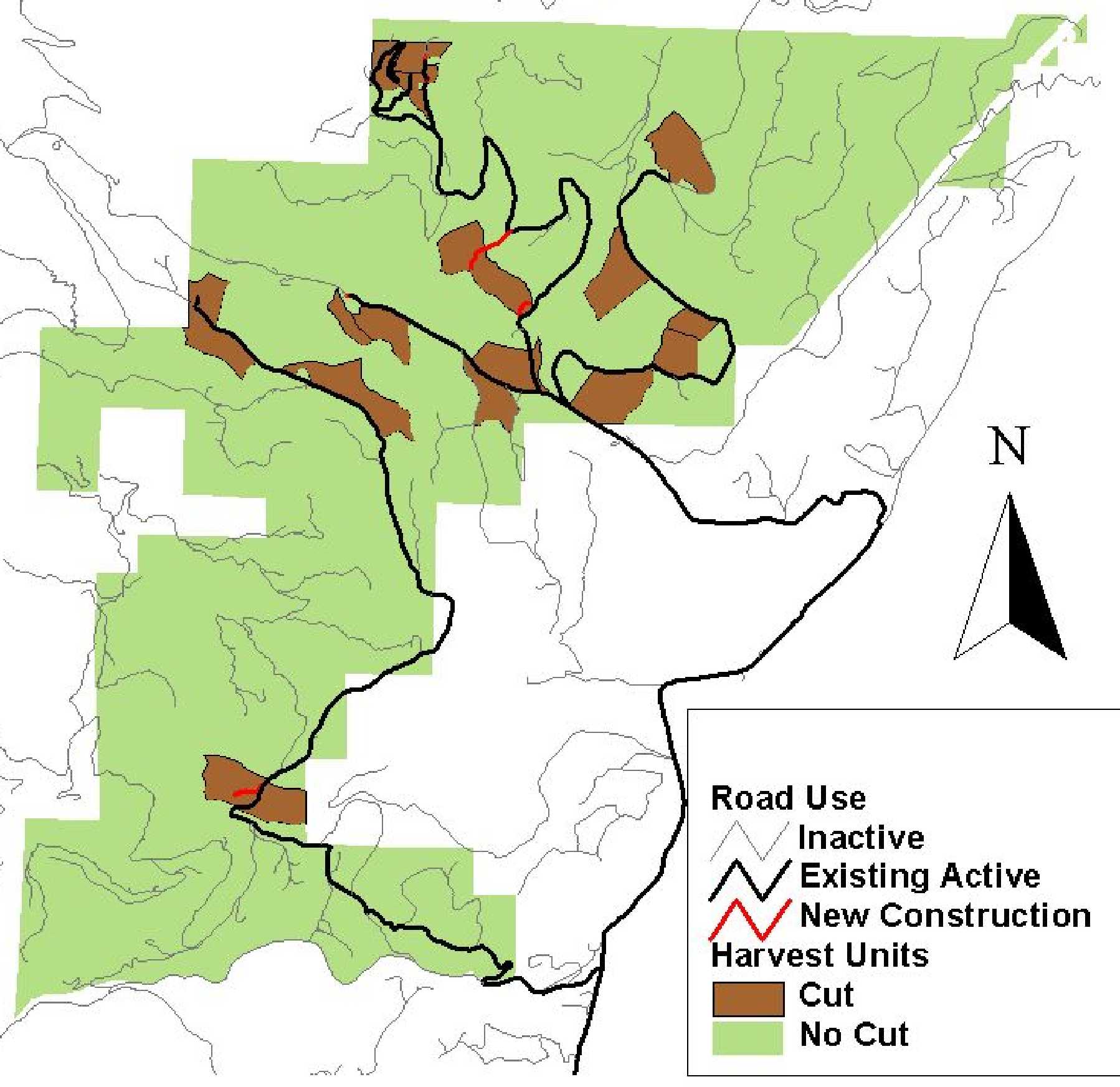
13.8.2 Period 2: 2004-2009
Figure
61. Road and harvest schedule based on SNAP analysis, 2004-2009.
In period 2 (Figure 61), the owl circles discussed previously are
still unavailable for management. As a result, harvest units are confined
to the eastern half of the Hoodsport planning area. This constraint
causes many new roads to be constructed due to the limited harvest
options. Two of these roads are of particular interest. The Wiki Ridge
road and the Powerline Road were both built in period 2 to access
much of the northeast corner of the planning area. These roads are
discussed in more detail in the Hoodsport Transportation Systems Report.
In accordance to the harvest volume goals provided by DNR, approximately
25,000 MBF were harvested in period 2. A summary of period 2 activity
is located in Table 26.
Table
26. Summary of period 2 road and harvest activities.
|
Managed Area
|
Harvest Volume
|
Existing Roads
|
New Construction
|
Revenue
|
|
880 acres
|
24719 MBF
|
15.8 miles
|
5.7 miles
|
$11.34 million
|
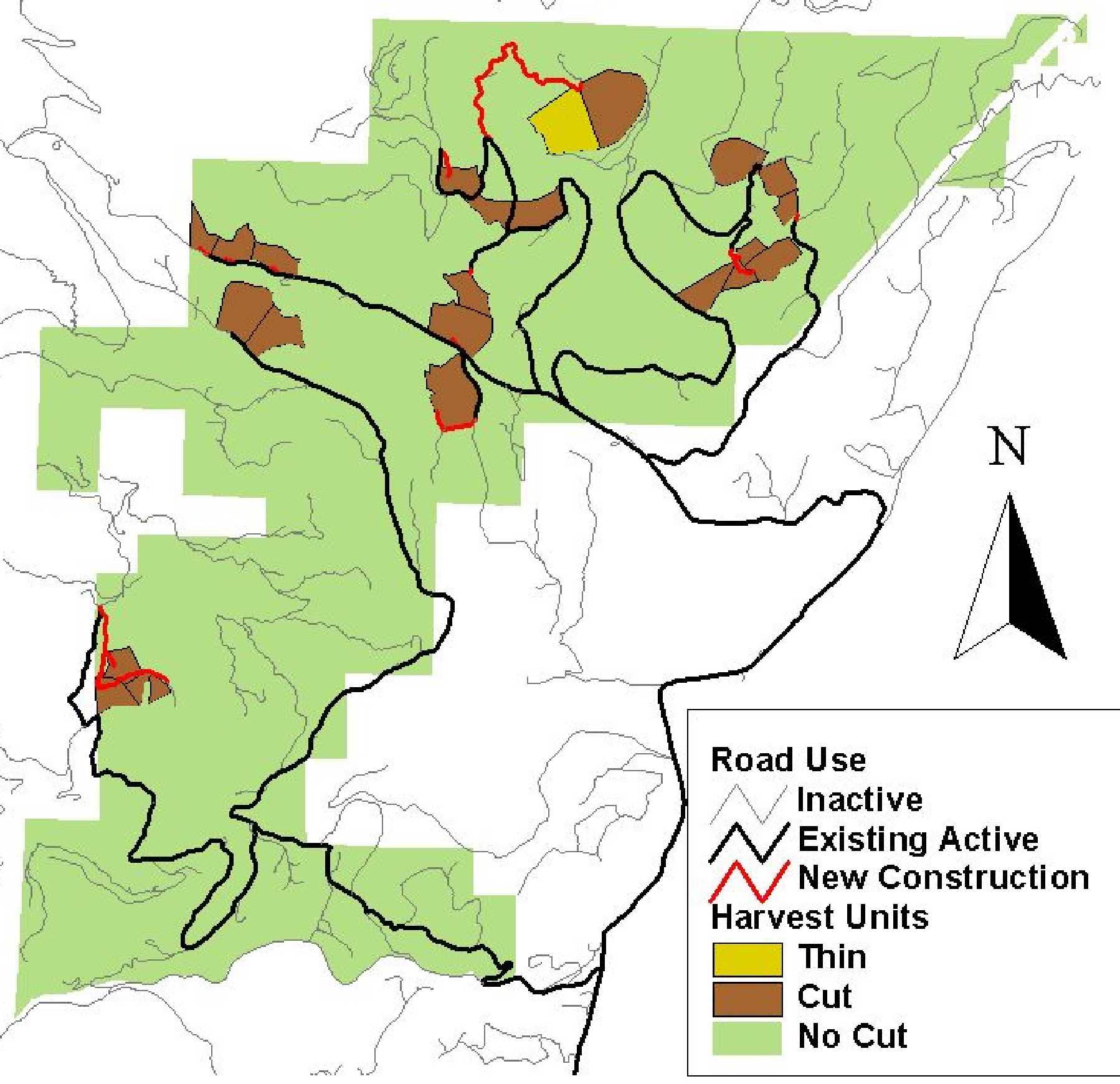
13.8.3 Period 3: 2009-2014
Figure
62. Road and harvest schedule based on SNAP analysis, 2009-2014.
Period 3 (Figure 62) signifies the end of the constraints due to
owl circles. This means that the western half of the planning area
can now be harvested. Note the very low amount of new road construction
(Table 27). This is due to the large amount of harvestable area added
in this period. There are many settings on existing roads that are
now ready to be harvested. Since they couldn’t be taken in previous
periods, they were selected for harvest now. As a result, new road
construction was limited to spurs.
Table
27. Summary of period 3 road and harvest activities.
|
Managed Area
|
Harvest Volume
|
Existing Roads
|
New Construction
|
Revenue
|
|
1040 acres
|
34701 MBF
|
16.4 miles
|
0.7 miles
|
$21.72 million
|
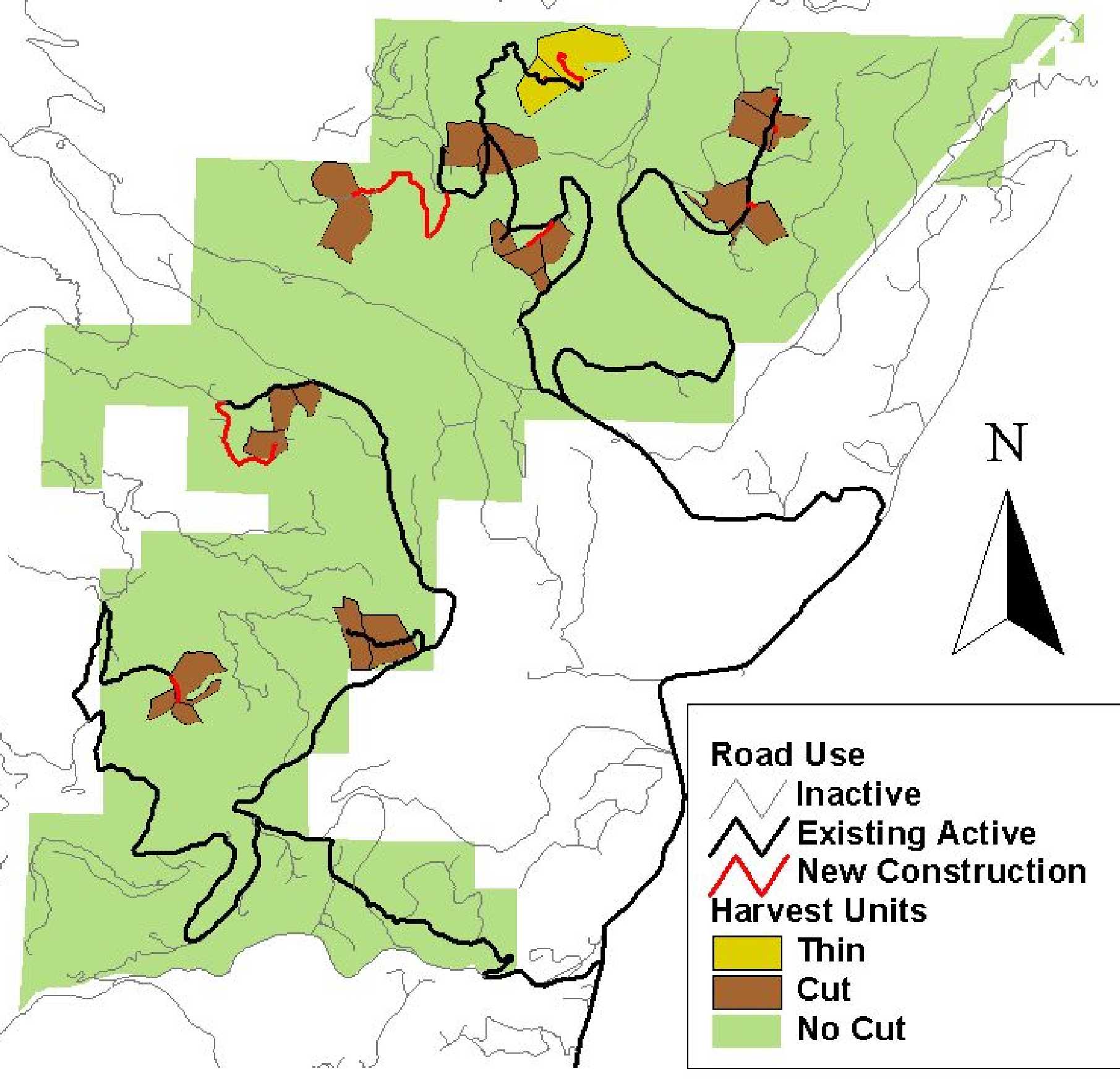
13.8.4 Period 4 2014-2019
Figure
63. Road and harvest schedule based on SNAP analysis, 2014-2019.
In period 4, SNAP chose to harvest a large block of Manke Lumber
land (see Figure 63). This is the half circle shaped group of settings
in the north part of the planning area. These settings were restricted
from harvest until period 4, and SNAP chose to harvest them as soon
as possible. Notice that in this period, one of the settings is commercially
thinned. The other half of the Manke land is commercially thinned
in period 5. This presents an interesting situation because DNR does
not currently own this land. According to this analysis, it would
be beneficial to DNR to explore the option of trading for this land
within the next 15 years. However, should Manke decide to harvest
the land before trading, or if either party opts against a trade,
some reworking of the period 4 and period 5 schedule will be necessary.
A summary of the activities in period 4 is included in Table 28.
Table
28. Summary of period 4 road and harvest activities.
|
Managed Area
|
Harvest Volume
|
Existing Roads
|
New Construction
|
Revenue
|
|
740 acres
|
44399 MBF
|
23.2 miles
|
3.6 miles
|
$30.61 million
|
13.8.5 Period 5 2019-2024
Figure
64. Road and harvest schedule based on SNAP analysis, 2019-2024.
In period 5 (Figure 64), the remainder of the Manke Lumber land
was commercially thinned. The Shirt Pocket road was still not entirely
built. It is reasonable to assume that the road would be built shortly
after 2024, but our analysis does not extend that far. The other major
roads designed by UW that were not used include Dynamite Ridge in
the southwest corner of the planning area, and the Hook Road in the
central section of the planning area.
In period 5, as in all other periods, the harvest volume goal was
met, or at least was within a reasonable tolerance. A summary of period
5 activities is provided in Table 29.
Table
29. Summary of period 5 road and harvest activities.
|
Managed Area
|
Harvest Volume
|
Existing Roads
|
New Construction
|
Revenue
|
|
700 acres
|
53500 MBF
|
21.3 miles
|
2.8 miles
|
$41.18 million
|
13.9 Harvest Volumes
The harvest volume goals for the North Hoodsport Planning Area increase
by 10,000 MBF for each period. In period 1, the goal is 15,000 MBF, and
it was easily exceeded by the DNR five-year action plan, even with the complications
of the owl circles. The goals were met in each period, concluding with 53,500
MBF in period 5. See Figure 65 and Table 30 for a comparison between the
harvest goals and the actual volumes harvested.
Figure
65. Harvest volume goals vs. actual harvest volumes by period.
Table 30.
Harvest volume goals and actual volumes achieved for each period.
|
|
Period 1
|
Period 2
|
Period 3
|
Period 4
|
Period 5
|
|
Harvest Volume Goals (MBF)
|
15,000
|
25,000
|
35,000
|
45,000
|
55,000
|
|
Actual Harvest Volumes (MBF)
|
22,731
|
24,719
|
34,701
|
44,399
|
53,500
|
13.10 SNAP Costing
The costs in Table 31 are from the SNAP analysis. An annual inflation rate
of 1% is assumed for all costs. The mill price of wood is assumed to grow
at 3%. Therefore, the costs and prices in period 5 are 2021 dollars, the
middle year of the period. The first period costs are in year 2001 dollars.
Costs in the Hoodsport planning area are relatively low due to the large
amount of existing road and the easy terrain.
Table 31.
Harvest costs and revenue by period from SNAP
|
Period
|
Volume (MBF)
|
Harvest ($/MBF)
|
Haul ($/MBF)
|
Construction
($/MBF)
|
Total Costs ($/MBF)
|
Mill Price ($/MBF)
|
Stumpage ($/MBF)
|
|
1
|
20731
|
84.01
|
38.31
|
13.90
|
136.22
|
538.35
|
402.14
|
|
2
|
24719
|
108.72
|
39.40
|
17.03
|
165.15
|
624.09
|
458.95
|
|
3
|
34701
|
54.59
|
41.29
|
1.61
|
97.49
|
723.50
|
626.01
|
|
4
|
44399
|
86.70
|
57.61
|
4.96
|
149.27
|
838.73
|
689.45
|
|
5
|
53500
|
135.06
|
63.65
|
3.97
|
202.68
|
972.31
|
769.64
|
13.11 Management of the Landscape
The percentage of the landscape that will be managed over time is shown
in Table 32. This 25-year plan manages approximately 40% of the landscape.
The amount of area being managed increases for each of the first three periods.
However, in period four, the managed area begins declining. This is the
time when growth rates for the timber catch up with the increasing harvest
volume goals indicated by DNR.
Table 32.
Percentage of the landscape under management by period.
|
Period
|
Managed Area (Acres)
|
Management as a %
|
Total Management of the landscape as a %
|
|
1
|
730
|
7%
|
7%
|
|
2
|
880
|
8%
|
15%
|
|
3
|
1040
|
10%
|
25%
|
|
4
|
740
|
7%
|
32%
|
|
5
|
700
|
7%
|
39%
|
13.12 Road Use
In Figure 66 and
Table 33
, the road use by period is shown. Road use is split into three categories:
existing inactive, existing active and new construction. Existing inactive
roads are the roads that currently exist on the landscape (including newly
constructed roads from previous periods) but are not being utilized in that
period. Existing active roads are the currently existing roads that are utilized
during the period. New construction signifies that a planned road is being
constructed during the period. Road decommissioning was not considered in
this data, so the total length of road on the landscape increases by the new
construction for each period. Road decommissioning is discussed in Chapter
14.
Figure
66. Road use by period. Road decommissioning was not considered here,
so the overall road use increases by new construction values. See
Table 33
for more information.
Table 33. Road use in miles
by period.
|
Road status
|
Period 1
|
Period 2
|
Period 3
|
Period 4
|
Period 5
|
|
Existing inactive
|
24.1
|
29.2
|
34.3
|
28.2
|
33.7
|
|
Existing active
|
16.3
|
15.8
|
16.4
|
23.2
|
21.3
|
|
New construction
|
4.6
|
5.7
|
0.7
|
3.6
|
2.8
|
|
Totals
|
45
|
50.7
|
51.4
|
55
|
57.8
|
Figure 67 is a representation of the road system for the Hoodsport planning
area at the end of the 25-year planning horizon. This includes both planned
and existing roads. Four categories were used to differentiate between planned
and existing roads, and used and non-used roads. Existing non-used roads,
displayed in red, are potential candidates for decommissioning. These are
discussed in more detail in Chapter 14.
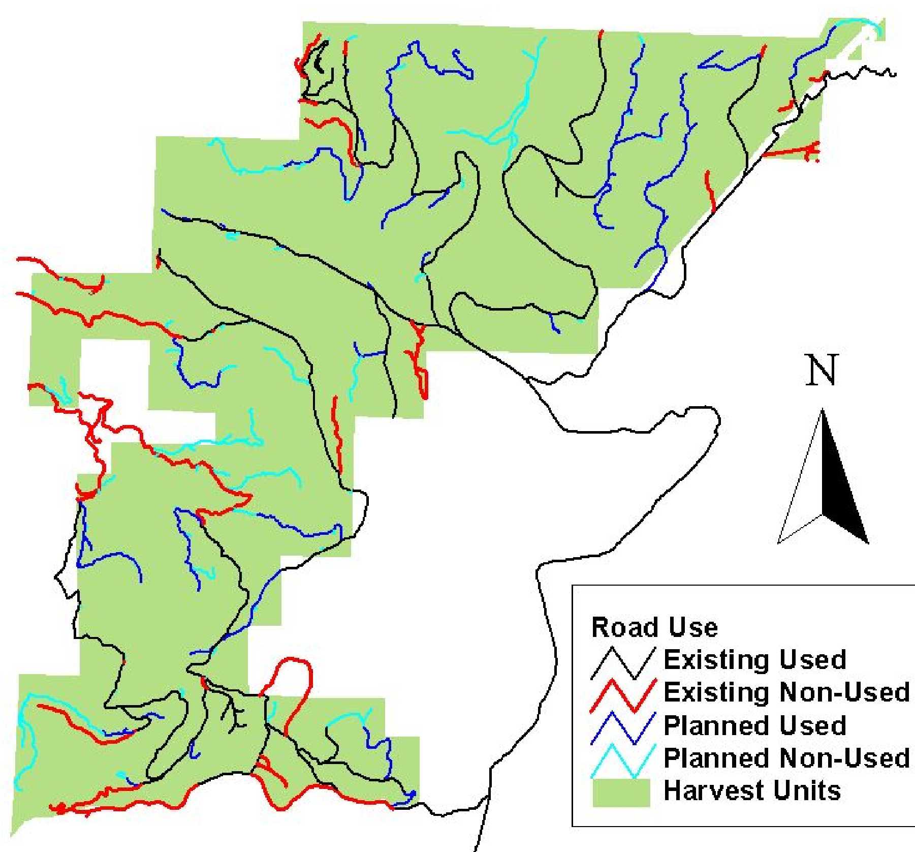
Figure
67. Final road pattern at the end of the 25-year planning horizon.
13.13 Final Recommendations
Based on the SNAP analysis, DNR’s proposed harvest goals over the next
25 years for the Hoodsport planning area are feasible. The result of this
harvest plan will be increasing revenue for every 5-year period over the
next 25 years. The standing timber volume increases for every period as
well, suggesting that revenue will continue to increase beyond the 25 year
planning horizon. The accuracy of this plan is only as good as the accuracy
of the input data, but we are relatively confident in the accuracy of our
inputs. Many of these were provided directly by DNR, and others were based
on reasonable assumptions.
The owl circles impacting the western half of the landscape will not be
overly limiting for the next 10 years. However, after that time, it will
be necessary to harvest within those areas to meet the harvest goals.
Manke Lumber’s inholding in the northern part of the planning area is also
an issue of interest. If possible, this land and timber should be acquired
within the next 15 years. If this is not possible, the harvest schedule
beyond 2014 must be re-analyzed.
In any case, the harvest and transportation plan for the next 10 years
allows for necessary habitat considerations and revenue production. Due
to changing political and social conditions, the final 15 years of the plan
will probably change in time, but DNR now has a large head start on any
necessary future analysis.
Back | Cover
Page | Table of Contents | Next