
Introduction to Geographic Information
Systems in Forest Resources |
Exercise: Vector
Analysis II
Objective:
- to learn the use of topological overlay tools
- to learn the use of buffering
- to learn the use of the ArcGIS model builder for streamlining work flows
- Perform drive
substitution to create drives L (CD) and M (removable drive).
- Make a directory for today's exercise
- Open a project
- Set the working directory
- Open ArcToolbox
- Append
- Clip
- Identity
- Union
- Intersect & Calculate Geometry
- Update
- Erase
- Buffering
Perform drive substitution
Perform drive
substitution to create the virtual drives L and M.
Make a directory for today's exercise
- Make a directory called M:\v_an_2 to store today's data.
- You may want to delete other data from your removable drive to free up space (except your Geodatabase).
I suggest keeping copies of all your old assignments somewhere (you can use
your dante account for this), but if you continue to store data on your removable
drive, you will eventually run out of space somewhere during the quarter.
If you still have the shapefile of the culvert inventory zones from the data
entry lesson, it will be used in today's lesson, so do not delete that, but
if you have already deleted your copy, you can download a copy during that
part of today's lesson.
Open a project
- Download the project v_an_2.mxd (use "Save As..."), and save
it in M:\v_an_2.
- Open the map document in ArcMap.
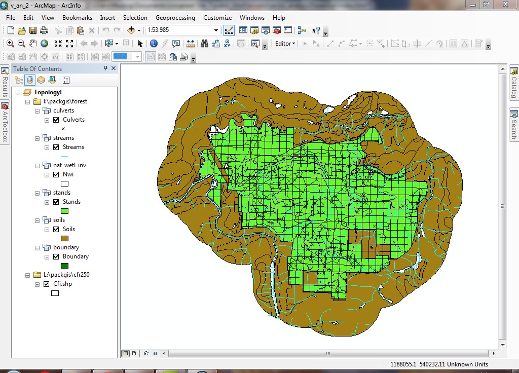
Set the working directory
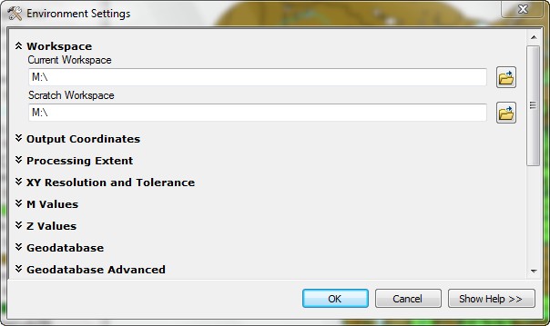
Make sure to Set Working Directory to the M:\.
Because you will be creating a number of new datasets, this will save the time
of you needing to navigate through a number of directories. (Geoprocessing > Environments.)
Open ArcToolbox
- Open ArcToolbox by clicking
 (It will take 3-5 minutes for ArcMap to load all tools)
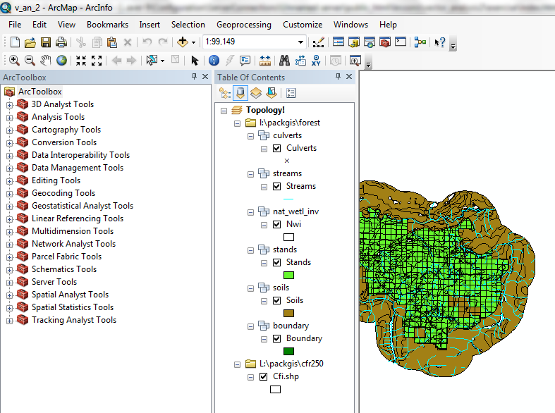
- If ArcToolbox is not docked in the GUI,double click at the top of the box and it will be docked:
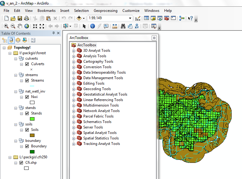
ArcToolbox is the application that contains all the overlay analysis tools.
Append
Appending layers is used to join together layers that represent the same features
on the ground, but whose spatial extents are contiguous (for example, data which
are tiled by township). Merge appends all spatial features into one layer, and
creates a single attribute table.
- Download the file sections.zip to M:\ (use "Save As").
This contains two shapefiles containing Public Land Survey System (PLSS) data
for the sections covering Pack Forest.
- Unzip the zipfile.
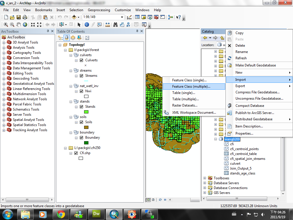
- Import the two layers (sections_north and sections_south) to your geodatabase: M:\NETID.gdb
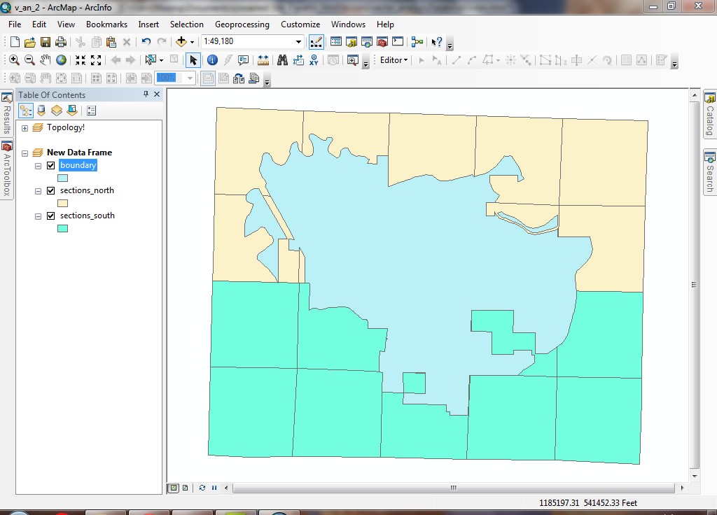
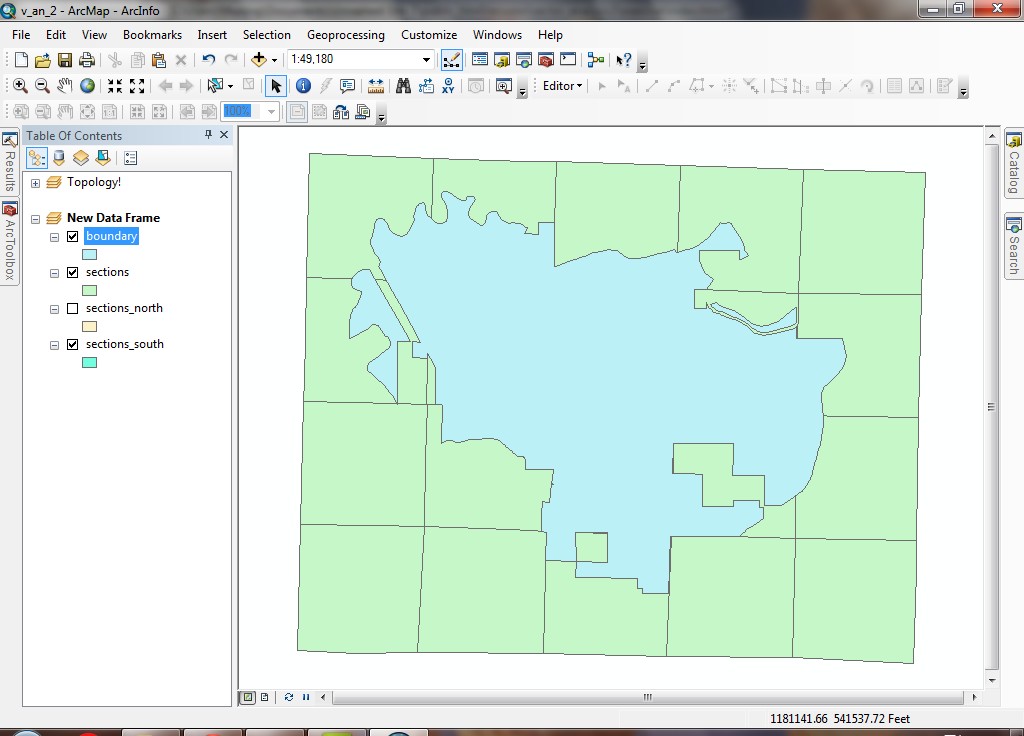
- Create a new data frame.
- Add the two layers (sections_north and sections_south) from your geodatabase (M:\NETID.gdb) and
the Pack Forest boundary (L:\packgis\packgis.mdb\forest\boundary).
- Change the display color for either the north or the south sections in order
to see the difference between the data sets.
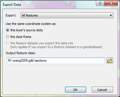
- Export the sections_north shapefile (right-click, Data > Export)
to M:\NETID.gdb\sections.shp. The reason for this is we will be appending
one data set onto another. In order to perform an append, it is necessary
to start with an existing data set, and then append other layers onto it.
- Use the Data Management Tools > General > Append tool. Select
sections_south from the Input Features dropdown. [Note: there
is another Append tool (Coverage Tools > Data Management >
Aggregate > Append) for use on coverage data sets; but in this case
we are using feature classes rather than coverages.]
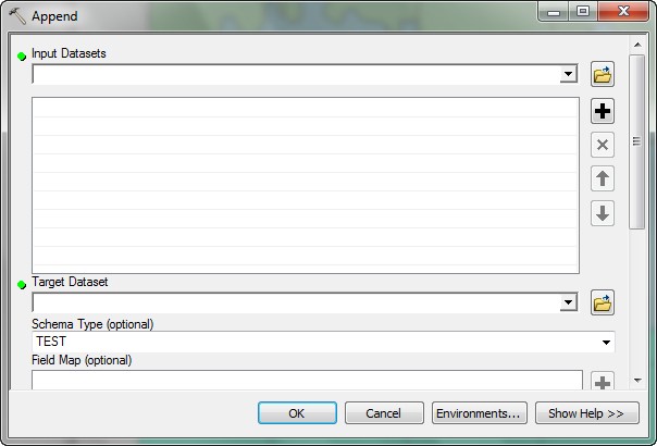
- Select sections in the Output Features control. Keep the default option of Test for
the Schema Type. Testing the schema type will compare the attribute
tables for the input data sets; if the attribute structures are not identical,
an error will be generated. Append starts with an exising data set that (usually) contains features, and adds features from the input data set(s) to that existing data set. In this case the features from sections_south will be appended to sections (which was originally created as a copy of sections_north)
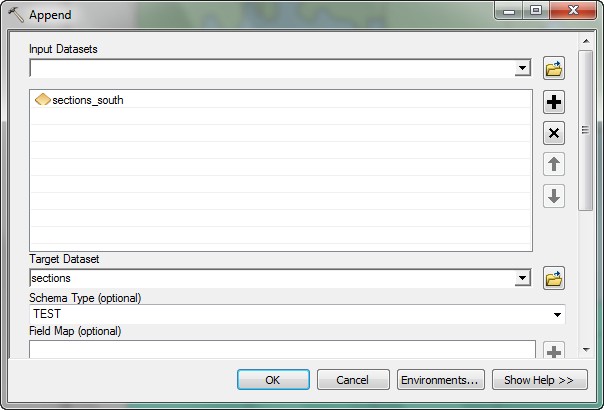
Click OK to start the process.
- After the process is complete, you can close the dialog.
- The newly appended data set will be added to the data frame:
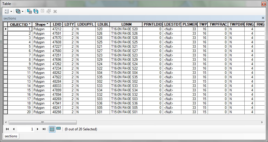
- Open the attribute table and scroll about halfway down. You will see that
all records have values, so not only were the shapes appended, but the records
were appended as well.
- Close the table and collapse the New Data Frame data frame to reduce
clutter in the Table of Contents.
You have just merged together two layers that were previously stored separately.
Now all features of both original layers are present in the new layer. You can
use this technique when you have adjacent datasets that represent the same features.
Clip
Back in Exercise 4,
we created a new layer of culvert inventory zones. When it was created, it was
made to go well outside the Pack Forest boundary.
Clip will now be used to limit the zones to the spatial extent of Pack Forest.
- If you do not have the culvert inventory zone shapefile saved, either digitize
one now (if you think you can do it quickly), or get it here (culv_inv.shp), as a self-extracting executable.
- Extract the Zip file and Import to your geodatabase M:\NETID.gdb after you download it. This will give
you a feature class called culv_inv.
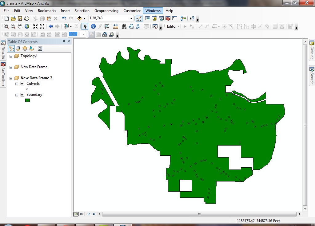
- With the <CTRL> key pressed, click the layers Culverts
and Boundary in the Topology! data frame. Right-click and select Copy.
Collapse the Topology! data frame to reduce clutter in the Table of
Contents.
-
Create a new data frame and change its name to
Culvert Inventory.
The new data frame will automatically be active.
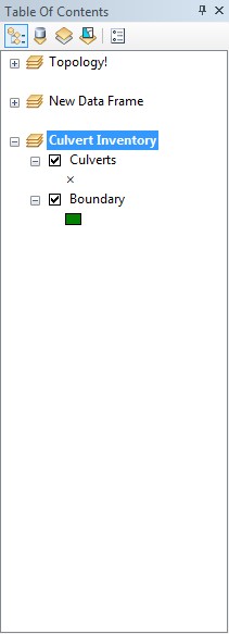
- Right-click the data frame's title and select Paste Layer(s). This
copies the Culverts and Boundary layers from one data frame
to another.
- Add the culv_inv layer to the data frame.
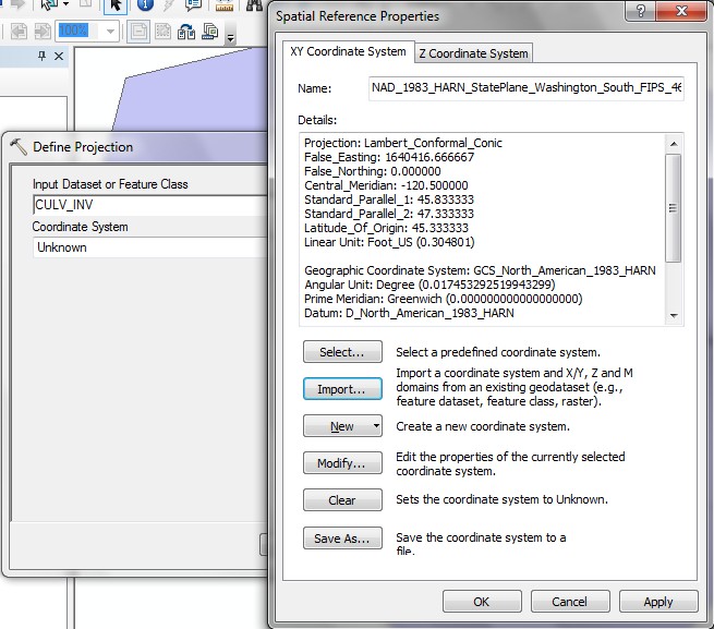
- Define the
projection (Data Management Tools-> Projection and Transformations
-> Define Projection) on the culv_inv shapefile to match the sections shapefile (Use "Import" instead of "Select"
when you define the projection). You now have several layers in your new data
frame.
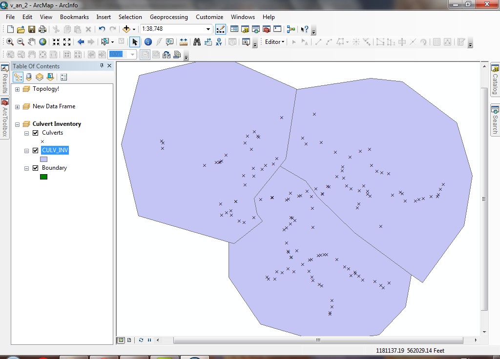
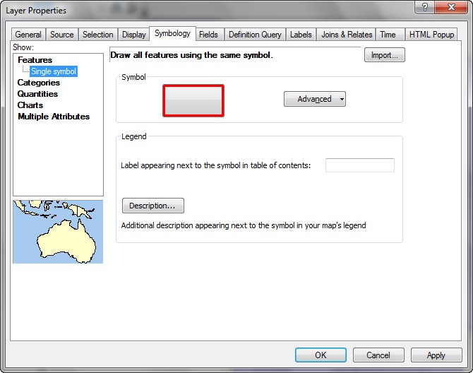
- Change the symbology of the culv_inv feature class by opening the layer's
properties and selecting the Symbology tab.
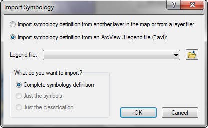
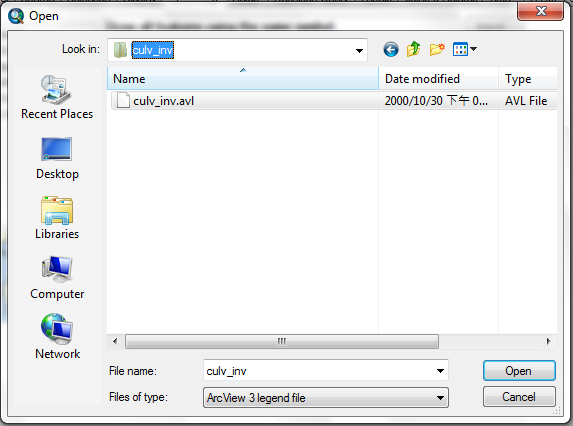
- Click the Import button. Choose to Import symbology definition
from an ArcView 3 legend file. A legend file specifies how a layer should
be displayed, including symbols and classifications. Browse to M:\..\culv_inv and select culv_inv.avl.
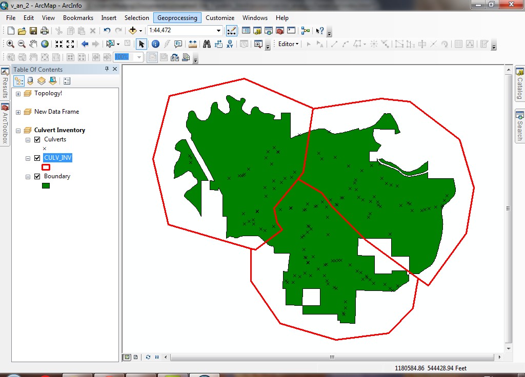
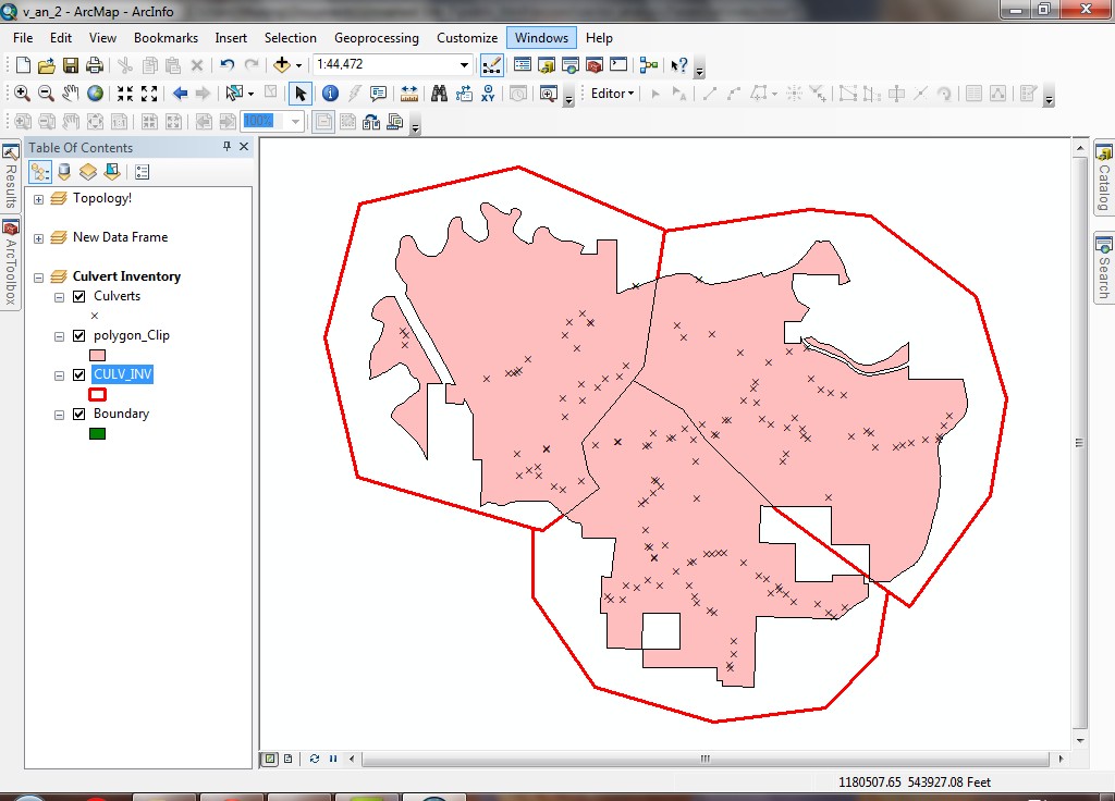
- This is a very simple legend file that will display the polygons as thick
red outlines.
- In the ArcToolbox Search tab, enter clip as the operation
to search for and click Search. A number of different tools will be
displayed. The one we will use is from theAnalysis toolbox, so double-click
it. You can search for tools in this way if you do not remember where tools
are in the ArcToolbox hierarchy.
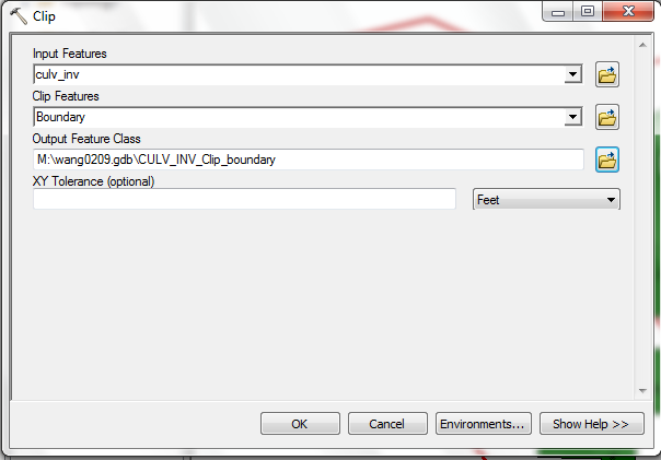
- The Input Features (that is, the features you want to clip) is
CULV_INV.
- The Clip Features (that is, the "cookie cutter") is
the Boundary.
- Enter the name of the Output Feature Class as M:\NETID.gdb\CULV_INV_Clip_boundary.
- Click OK and the process will start. After a few moments the process
will complete, after which you can Close the dialog.
- The new layer will contain the same zones, but will be clipped down to the
same overall spatial extent as the entire Forest.
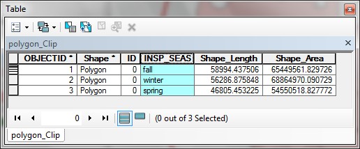
- Open the attribute table of the new shapefile. Note that the attributes
from the original data source are maintained in the clipped version.
You have just used a clip to limit the spatial extent of one polygon
layer based on the spatial extent of another polygon layer. Use this technique
when you need to limit one layer by the outer boundary of another. Sometimes
you need to perform mapping or analysis of a subset of your data. Rather than
using the entire larger dataset, you can limit the extent in this way.
Identity
Use identity to both limit the spatial extent of the output by the extent of
the identity layer, but also to carry all attributes from both input datasets
onto the output data set.
You will be creating a new National Wetlands Inventory layer that is limited
to the Pack Forest boundary extent, but which is also coded for all forest stand
attributes.
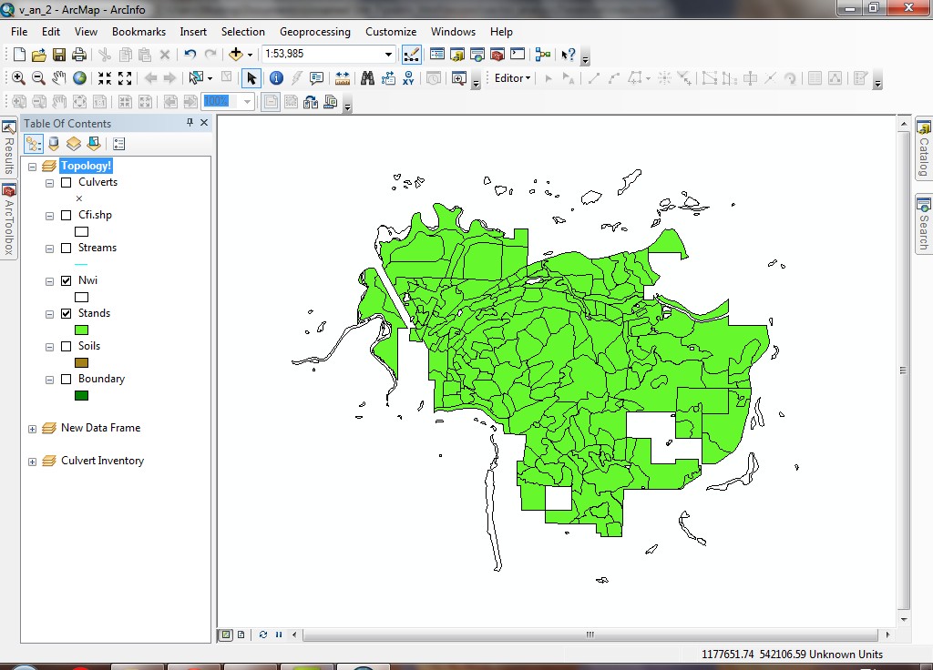
- Collapse the Culvert Inventory data frame and make the Topology! data frame active, and turn on only the Nwi and Stands layers.
- Open the attribute tables for Nwi and Stands. Note the field
names and the values present.
- The Identity is located at Analysis Tools\Overlay\ in ArcToolbox.
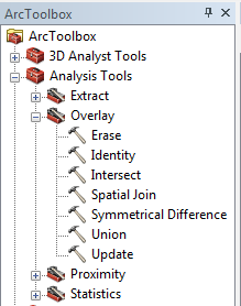
- Double-click on the entry to open the tool.
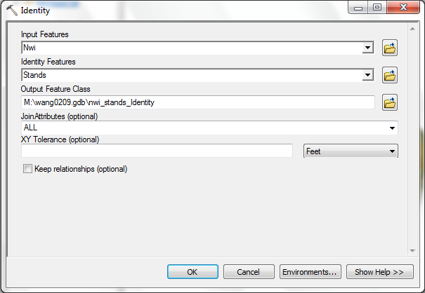
- The Input Features are the Nwi polygons;
- Set the Identity Features to Stands;
- Set the Output Feature Class to M:\NETID.gdb\nwi_stands_Identity
The order of Input and Identity layers matters; if you switch the layers
used for these, the output data set will have different geometry.
- Close the dialog after the process finishes.
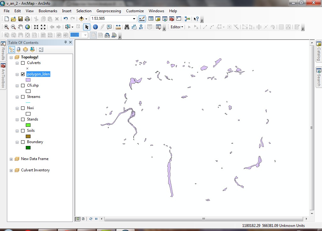
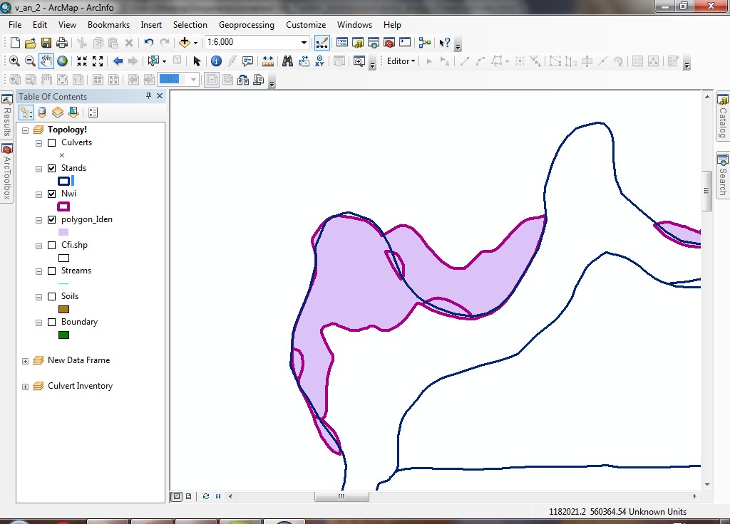
- The new data set looks like the original NWI polygons. But zoom into a location
indicated in the image below:
- Experiment with turning layers on and off and you will see how the spatial
properties of the original NWI data set have been altered.
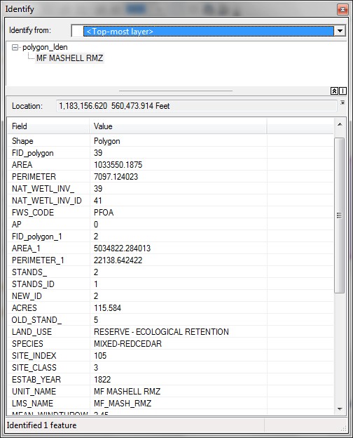
- Only click on Nwi and Stands layers, make they visible. Use the Identify tool and click on an NWI polygon that overlaps with
one of the stand polygons. You will see that the polygon has all of the attributes
from both parent data sets.
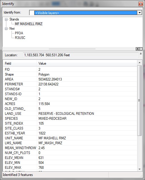
- Then click on the new idenitify layer, and then identify one of the polygons. You will see that
all values there are from stands and Nwi layers:
Exactly what are the area measurements for these polygons? Fortunately, the
area values will show up automatically since we are using geodatbase to save our data (Field Name: Shape_Area). If you are using the the shapefile as your data format, you will need to use "Calculate Geometry" from the attribute table of this layer to update the Area values.
You have just created a new layer based on the overlap of two input layers.
If any areas overlap between the two input layers, the polygons representing
those areas have attribute values from both inputs. Where there is no overlap,
only the input attribute values exist. This technique is used to identify areas
that are common between two layers, but only the coordinate data from the input
layer exist in the output, and where shapes overlap, features are split.
Intersect & Calculate Geometry
Contrast Intersect with Identity. The same layers will be used, Nwi
and Stands, but instead of an Identity, use an Intersect.
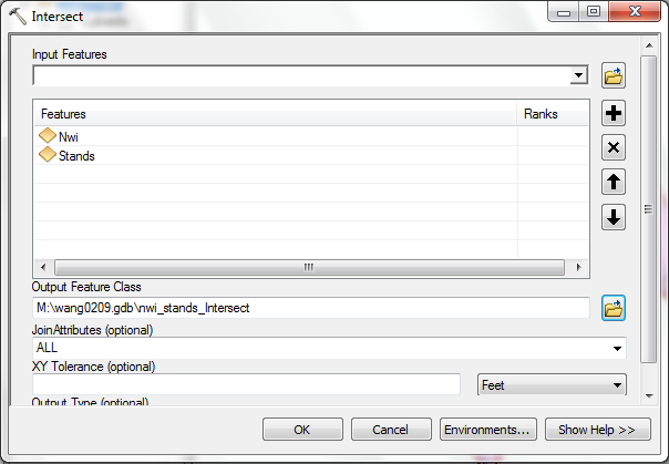
- Open Analysis Tools > Overlay > Intersect.
- Again, select NWI and Stands as the Input Features
.
- The Output Feature Class can be called anything you like, but
I suggest using M:\NETID.gdb\nwi_stands_Intersect.
- After you have selected both layers, click OK. In this case, the
order in which you select layers does not matter, because the output will
only contain geometry that is clipped to the common geometry of all
input data sets. Note that you can also get the intersection of more than
just two data sets.
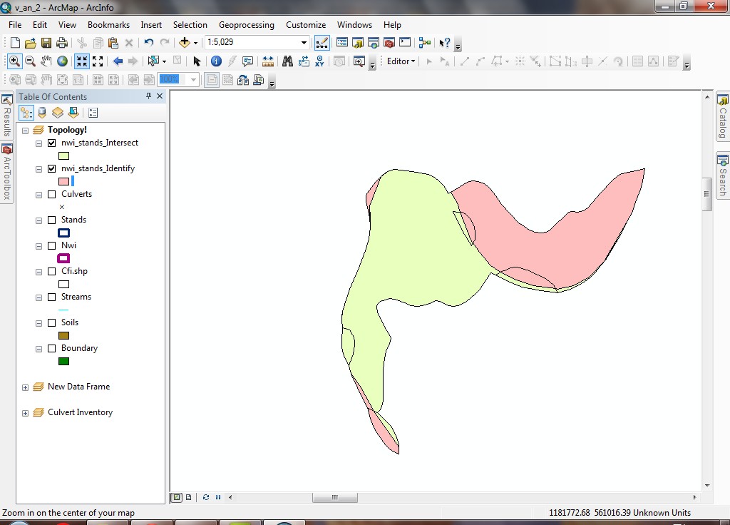
You can see how the Identity output has the same overall geometry of the Nwi
data set, whereas the Intersect output is clipped to the common areas of both
Nwi and Stands.
- Open the attribute table for the new layer. Note that fields exist for
both input layers, but the geometry is not correct, try to recalculated the geometry for next step.
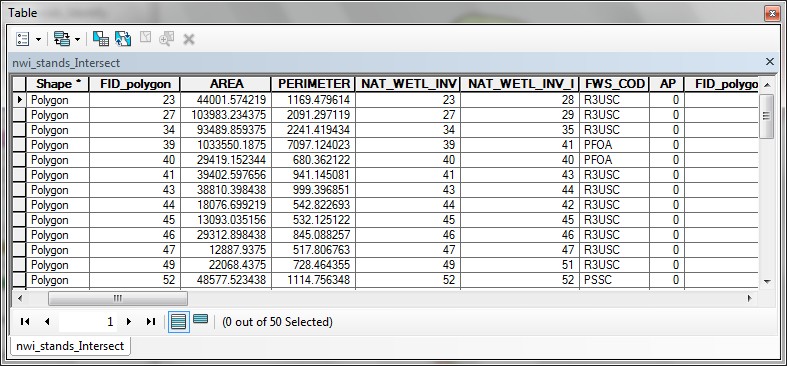
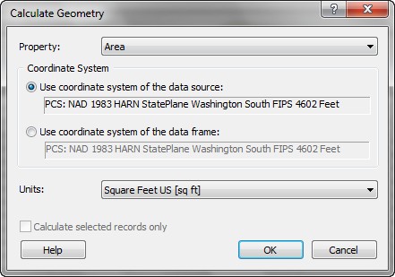
- Calculate Geometry: Right click on the geometry attribute field (length, area, perimeter, XY coordinates), choose Calculate Geometry, and click yes to open the tool.
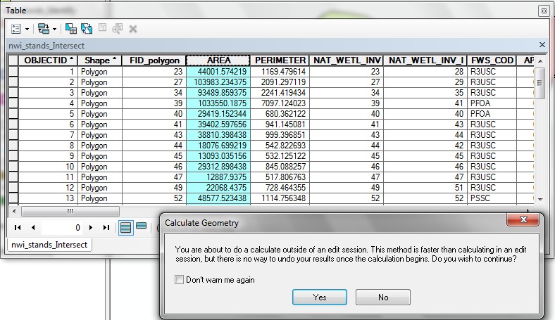
- Choose the right geometry you want to recalculate and updated (for example, here is AREA), choose the new unit you want to manipulate (or keep it same as the layer projection), and then click OK.
- You can compare the new value in the table versus the previous table you had in step 4, the value is totally different, and you need to calculate geometry all the time once you use ArcToolbox to perform any vector analysis tools.
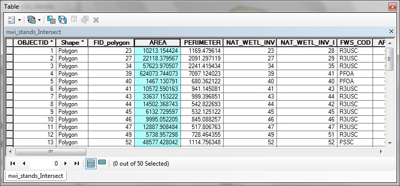
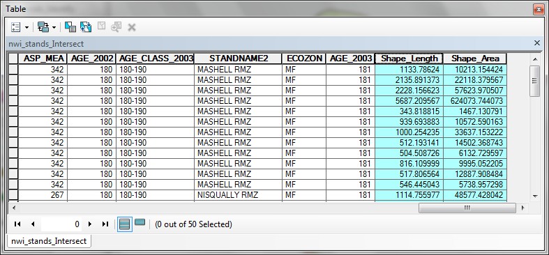
- If you saved your
new layer into Geodatabase, the geometry will be update automatically into new field, called "Shape_Length" & "Shape_Area" in the end of table, you do not have to update by yourself, and the unit is as same as layer projection.
Plus, Identity and Intersect are similar in what they do, except that the output
spatial extent differs. Where there is no overlap, polygon areas are deleted.
Union
Union the Soils polygon layer and the Stands polygon layer.
- In ArcToolbox, open the Union tool. Like Intersect, the order of
input and overlay does not matter.
- In ArcMap, use the <CTRL> key and select both the Soils
and Stands layers. Drag these into the Features control in the
Union tool.
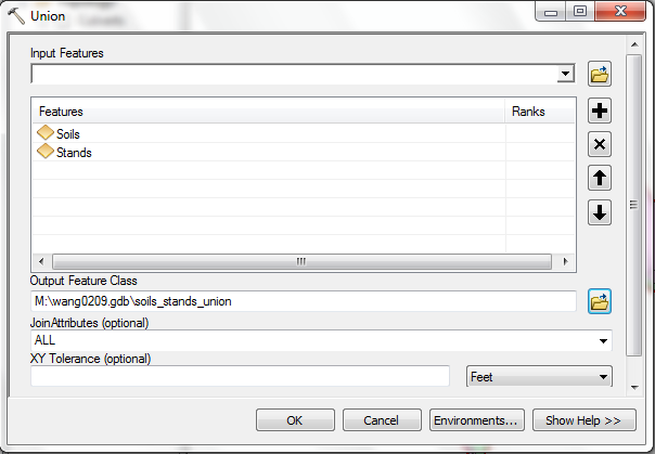
- Rather than entering a name for the output data set, click the Browse button
and navigate inside the geodatabase. Enter the name soils_stands_union
for the output feature class.
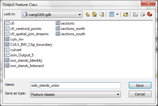
- Click Save for the Output Feature Class and OK the tool.
- Note that the new feature class combines the geometries from both input
layers.
- Identify one of the polygons to view its attribute structure. Note
how both parent layers' attribute fields and values appear in the new layer's
table.
- Open the table for the new layer and scroll all the way to the right.
Note the fields Shape_Length and Shape_Area. These represent
perimeter and area for each polygon. These values are automatically generated
and updated. Note that the original Area and Perimeter fields
exist; because the feature geometry has been altered, these fields are no
longer valid (you can easily see this by looking at the identified feature
above: AREA = 6279539 ft^2, Shape_Area = 812053 ft^2).
Union is similar to Identity and Intersect, but all features from all input
layers are preserved in the output. Remember that in Identity, only the geometries
from the input layer are preserved; in Intersect, only common geometries are
preserved.
Identity and intersect can pair polygon layers with point or line layers as
well as with polygon layers.
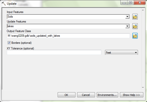
Update
Use Update to replace the contents of one polygon layer with the contents
of another. Here, we will update the Soils layer with the Lakes
layer. This can be useful if you have a newer or more accurate dataset that
you would like to use to replace parts of an existing dataset.
- Add the L:\packgis\packgis.gdb\forest\lakes layer to the data frame.
- Open the Update tool from ArcToolbox.
- Drag Soils from ArcMap into the Input Features control.
- Drag lakes polygon to the Update Features control.
- Browse to the geodatabase and set the name of the new data set to soils_updated_with_lakes.
- After the process completes, zoom in to an area where lakes exist (see
image below).
- You can see the original Soils polygons show water features (if
you change the symbology to show unique values based on SOIL.NAME
this becomes apparent).
- The new data set has its geometry updated with the features from the
lakes polygon layer.
- Select one of the features. In this case, the new feature's geometry
originates from the lakes polygon layer, but the area the new polygon
occupies was originally an area of overlap with SCAMMAN soils.
- Update works to add the new overlapped polygon or features
to another layer and output a new layer named soils_updated_with_lakes.shp.
Now you can see soil layer has lake polygon information. The selected
lake polygon is a part of soil layer now.
You have just replaced parts of one polygon layer with polygons from another
layer.
Erase
Contrast Update with Erase. Erase removes the overlapping features
from the input layer. In this example, remove the Lakes areas completely
from the Soils layer.
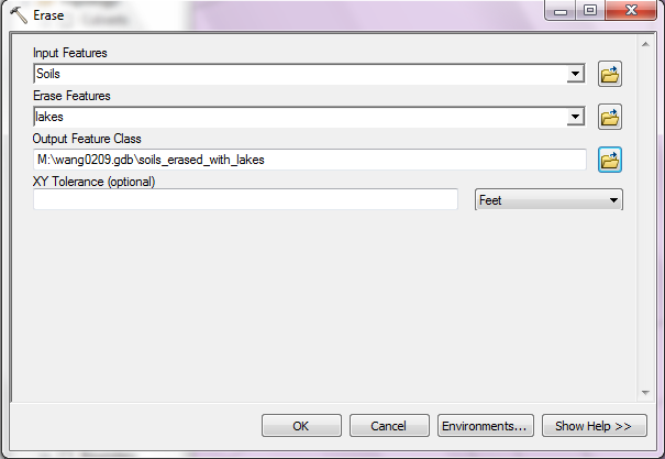
- Open the Erase tool.
- The Input Features is set to Soils.
- The Erase Features ("cookie cutter") is lakes polygon.
- Place the output in the geodatabase as soils_erased_with_lakes.
- It is obvious what Erase does by viewing the new data set.
The places where lakes were have been completely deleted from the Soils
layer.
You have just deleted parts of one polygon layer using polygons from another
layer. Anywhere there was overlap, areas have been removed.
Buffering
Buffering creates a new polygon layer at either constant or variable distance
from features in an input layer. In this exercise you will create variable-width
buffers around roads based on the road type. You will associate a buffer distance
for each road segment by creating a summary table and temporarily joining the
summary table to the roads table. This is a preferred method because it does
not permanently alter the roads table; once the buffer is complete, the join
can be broken.
- Create a new data frame called Road Buffering.
- Add the Roads layer from L:/packgis/packgis.mdb/forest/roads to this data frame.
- Create and alter a summary table from the roads table.
- Open the attribute table for the layer.
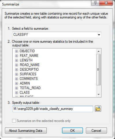
- Perform a summary based on the CLASSIFY field.
- Do not specify any summary statistics (this will create a simple table with a record for each road class).
- Specify the output table as M:\NETID.gdb\roads_classify_summary.
- Add the table to the map.
- Open the table.
- Add a field called buff_dist.
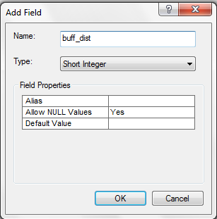
- Using the Editor toolbar and select Start Editing. Update
the values of the buff_dist field as shown here. These are the
buffer widths that will be applied to each road use type, for example,
HIGHWAY road features will be buffered by 30 feet.
- After your edits are complete, stop editing (and save your edits).
- Join the summary table onto the roads table using the CLASSIFY field
as the joiner.
- Now you will see that the roads table has the buff_dist field.
Remember that joins are temporary, so after the buffer is complete you
can remove the join and your roads table will be unaffected.
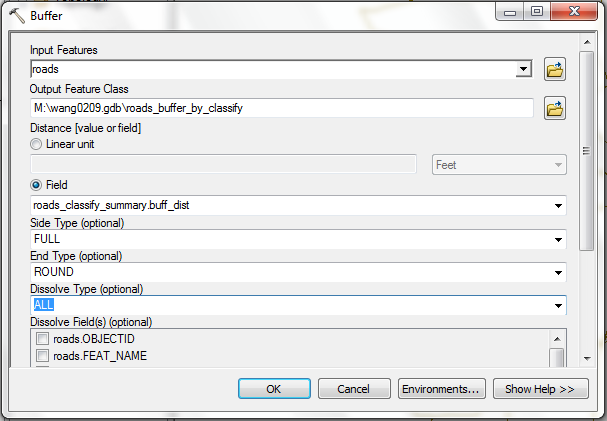
- Open the ArcToolbox > Analysis Tools > Proximity > Buffer
tool.
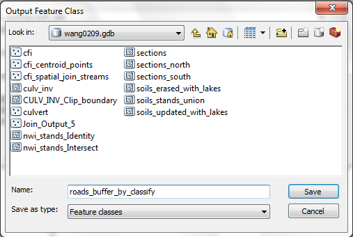
- The Input Features should be set to roads.
- Set the Output Feature Class to roads_buffer_by_classify
within the geodatabase.
- Select the Field radio button for specifying the buffer distance. Select the joined buff_dist
field. This instructs ArcGIS to use buffer values on a feature-by-feature
basis, controlled by the value of the buffer distance on each feature's
record.
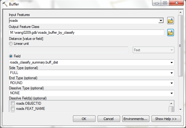
- Scroll down and make sure to choose Dissolve to ALL
(but be aware of what this does by looking at Show Help).
- Click OK to start the buffer process. After a few moments
the process will be complete. Zoom in to view the output. You will
see that different roads are buffered at different distances.
You have just created variable-width buffers of road features. The buffers
define an area that is a discrete distance from each buffered road segment.
Any vector feature can be buffered in this way. It is common to buffer features
in order to delineate areas of influence, or to create areas of altered land
use. For example, under current forest regulations, depending on the stream
class, different activities are permissible at different distances from the
stream channel.
REMEMBER TO TAKE YOUR CD AND REMOVABLE DRIVE
WITH YOU!!!!
Return to top
 |
|
TThe University of Washington Spatial Technology, GIS, and Remote Sensing
Page is supported by the School of Forest Resources
|
|
School of Forest Resources
|
 UW
Home
UW
Home