
Introduction to Geographic Information
Systems in Forest Resources |
Exercise: 3D and Surface Modeling and Analysis
Objectives:
- to derive slope and aspect surface grids from an elevation grid.
- to use surface analysis functions.
- to use 3D display functions.
- Perform drive
substitution to create drives L (CD) and M (removable drive).
- Create a new map document
- Add surface model data layers to a data frame
Alter the legend for a TIN layer
- Derive slope and aspect grids
Derive a slope grid
Create a percent slope grid
Create an aspect grid
- Find steepest descent path
- Analyze line of sight and create surface profiles
- Create a viewshed
- Create surface profiles from line features
- Create a 3D scene
- Display other (non-elevational) data in 3D
Perform drive substitution
Perform drive
substitution to create the virtual drives L and M.
Create a new map document
- Start ArcGIS.
- Create a new directory, M:\3d to
store this lesson's data.
- Create a new map document, rather than opening an existing one. Save
the document as M:\3d\3d.mxd.
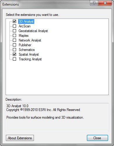
- Enable the 3D Analyst and Spatial Analyst extensions from "Customize > Extensions..."
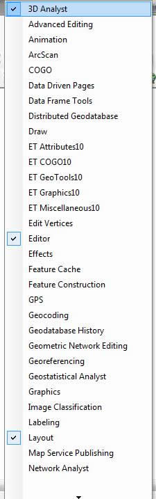
- Enable the 3D Analyst toolbar (Right click mouse from the meanu bar)
Add surface model data layers to a data frame
View a TIN layer and alter its symbology
- Rename the Layers data frame to
TIN. (More information about TIN format: http://en.wikipedia.org/wiki/Triangulated_irregular_network)
- Add the dem grid data source from the L:\packgis\forest directory.
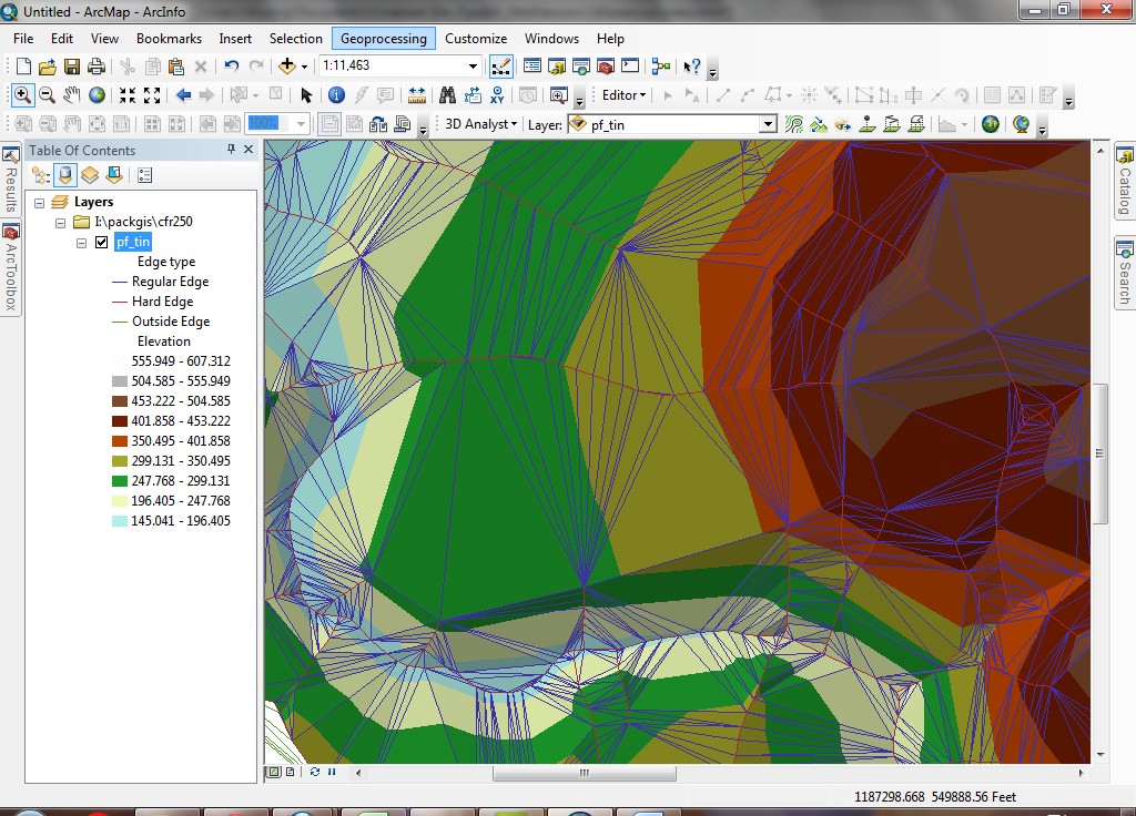
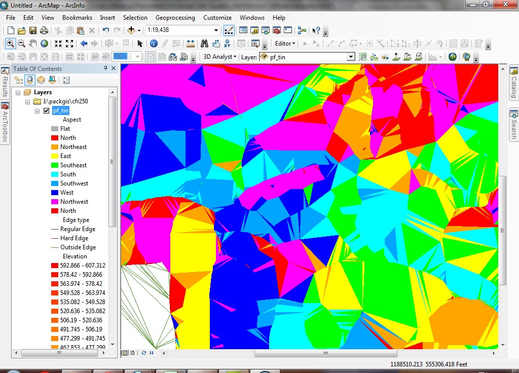
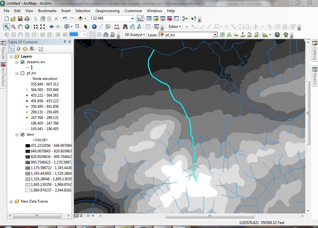
- Add the pf_tin (TIN Data Source, on the CD in the L:\packgis\cfr250
directory). The Pf_tin layer will load with random-colored breaklines,
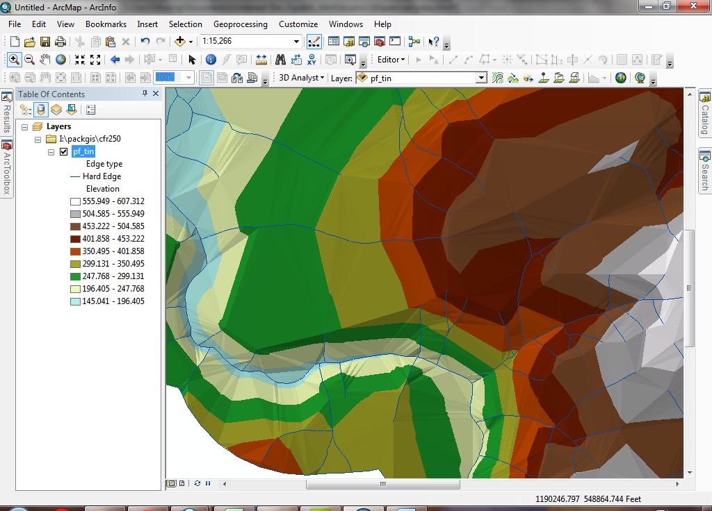
but with a green > red > white elevation fill legend. Zoom into the
area shown by the red box below.
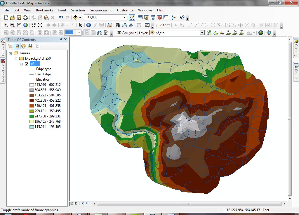
- Note the hard edges. Hard TIN edges for this data set are enforced
by stream lines.
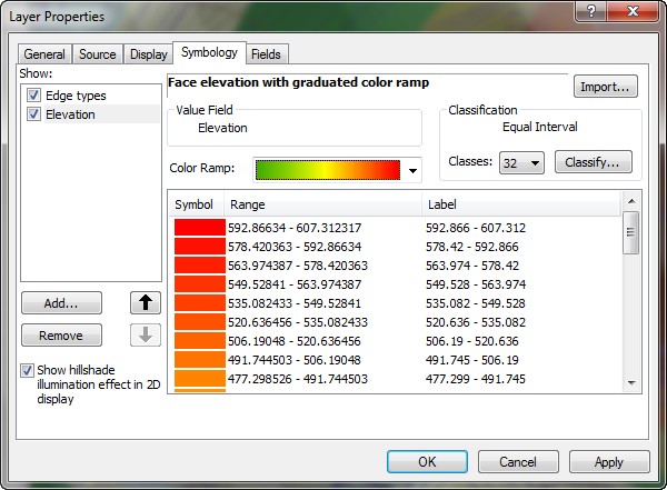
- (NOTE: In MGH 044, since the map server is done and can not be fixed so far, if you can not run the "Symbology", just read through the exercise, but you can finish your this lab exercise either in Suzzallo GIS lab or your own laptop or desktop.) Open the symbology properties for Pf_tin. Note there are two different
feature types listed (Edge types and
Elevation). The Symbology Function may not be able to perform due to the lab computer issue, if you are running into the difficulties, just read through it (till Step 15).
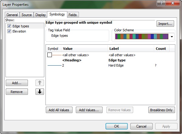
- With the Edge types features selected
(note the difference between selected and checked!), click Add All Values. TIN triangles are composed
of a number of different edge types. Adding all values will show all the
edge types for the TIN. For more information on TIN creation and breaklines,
see ArcGIS 's on-line documentation.
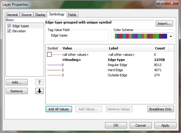
- Now you see all the different edge types. Note that in some places the
triangles are very small, whereas in other places the triangles are very large. Where the surface is more convoluted there are more and smaller triangles, but
where the surface is more simple, it can be represented with fewer large triangles.
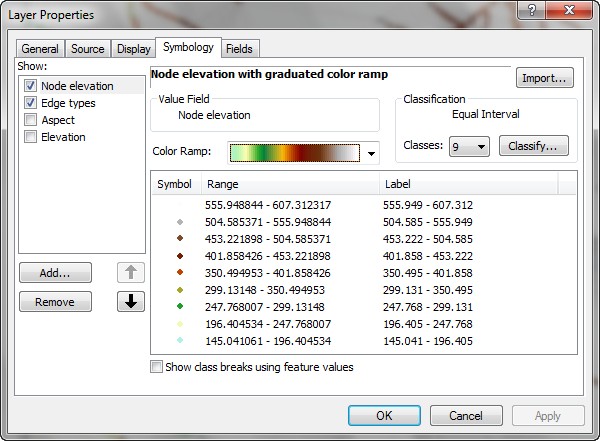
- Select Elevation. Alter the
number of classes to 32, select the
green-yellow-red color ramp, and uncheck
the Show hillshade checkbox.
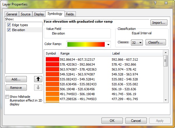
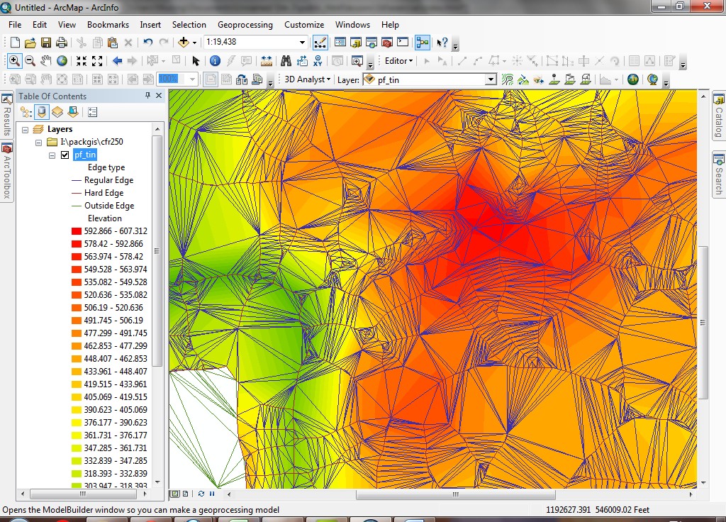
Now you can see more elevational variation. But without artificial hillshading
it is difficult to determine the form.
Recheck the Show hillshade checkbox
to see the landform
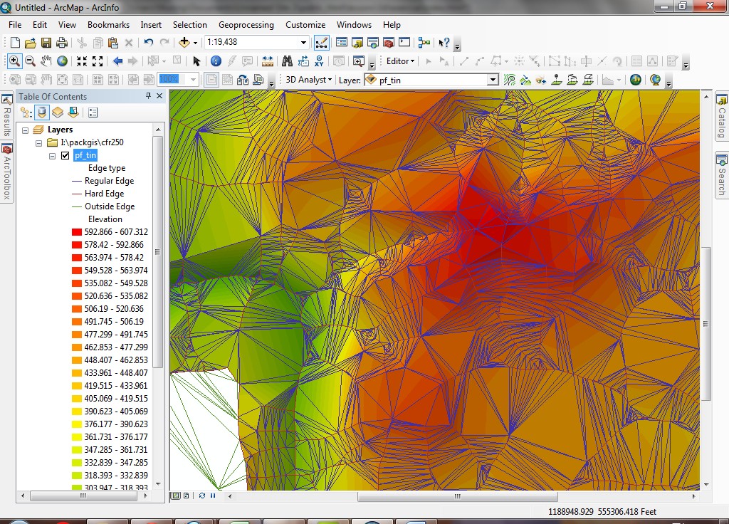
Do you see how shading makes a big difference in the appearance of surface
models? Shading is what allows the eye to interpret a surface as a 3-dimensional
object.
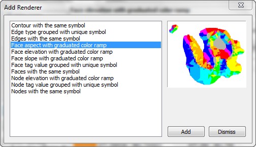
- Open the symbology properties again and click the Add button.
There are several additional choices for how to render (display) the 3D TIN
data.
- Select Face aspect.... Aspect,
or slope direction, is the compass bearing for each triangle face. Imagine
if you dropped a bowling ball on a triangle edge and measured the compass
angle of the ball's trajectory; this is the aspect value. And uncheck "Elevation".
- Do you see how the location circled below has triangles facing northwest? If you can imagine the erosional effect of a stream, this should make intuitive
sense.
- Add another renderer (Properties > Symbology
> Add). This time select Node elevation...
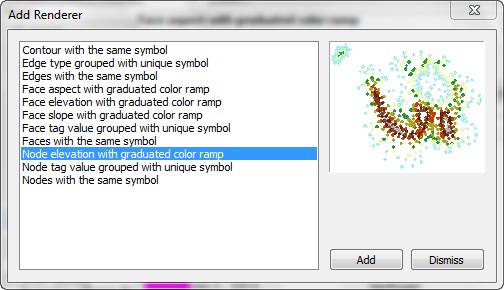
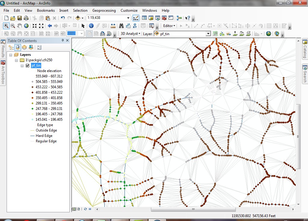
- Alter the drawing order by selecting the Node elevation type and clicking the
 button.
- You can now see the individual vertices (nodes) that define each triangle.
- Compare the TIN elevation histogram against the dem histogram: The histogram from the dem layer is shown directly below for the purpose of comparison.
 dem histogram
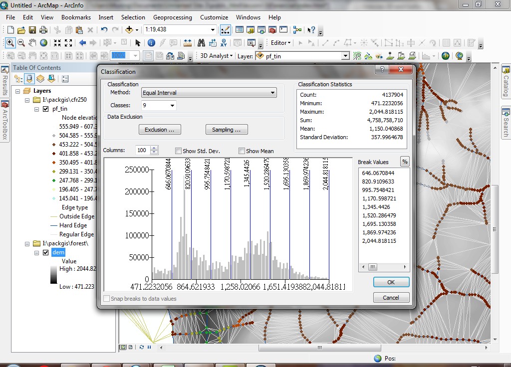
View the histogram from TIN elevation (open the Properties > Symbology > Classification dialog for the TIN).
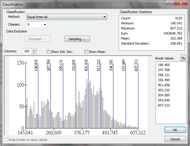
The overall bimodal distribution is similar between the two data sets. But the data sources that created the two different surface models are different.
You have just loaded and altered the legend properties for a TIN. Why do you
think each triangle appears with a single shade? What feature of the TIN model
makes this so?
TINs are used in addition to grids as data sets representing surfaces. Certain
surface modeling and analysis functions in ArcGIS act only on TIN surfaces,
and not on grid surfaces.
Derive slope and aspect grids
Derive a degree slope grid
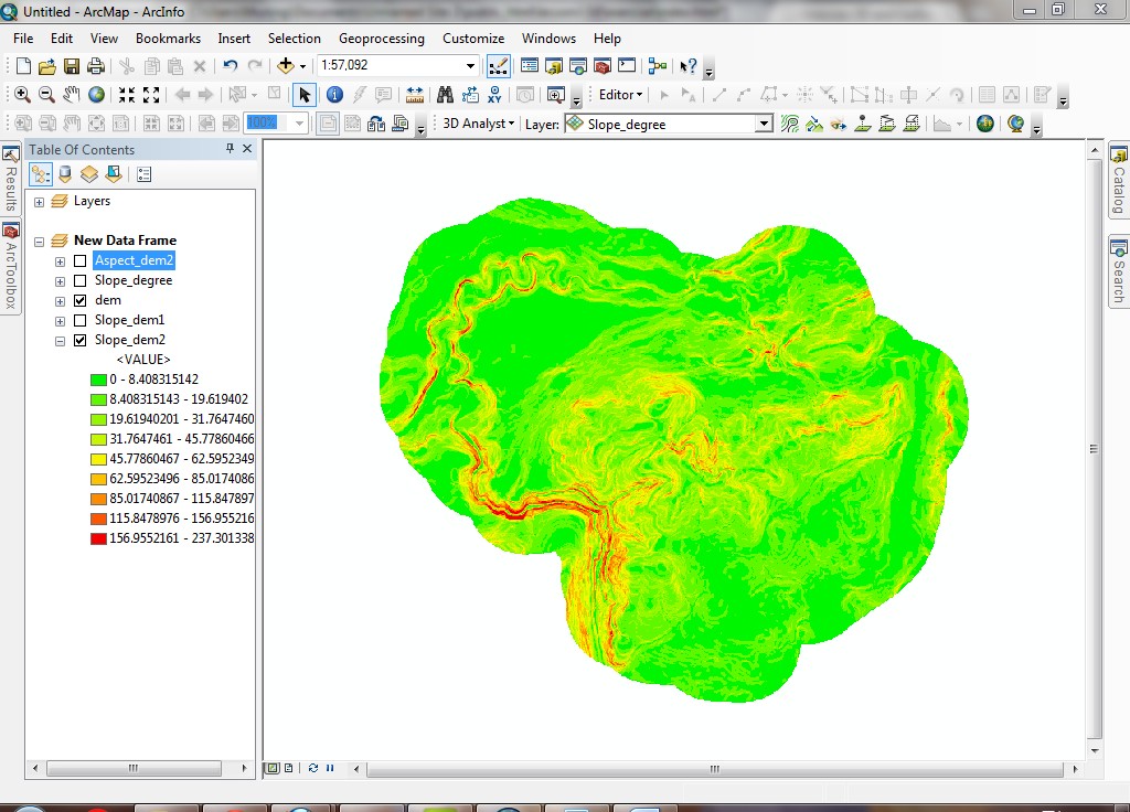
- Zoom back out to full extent.
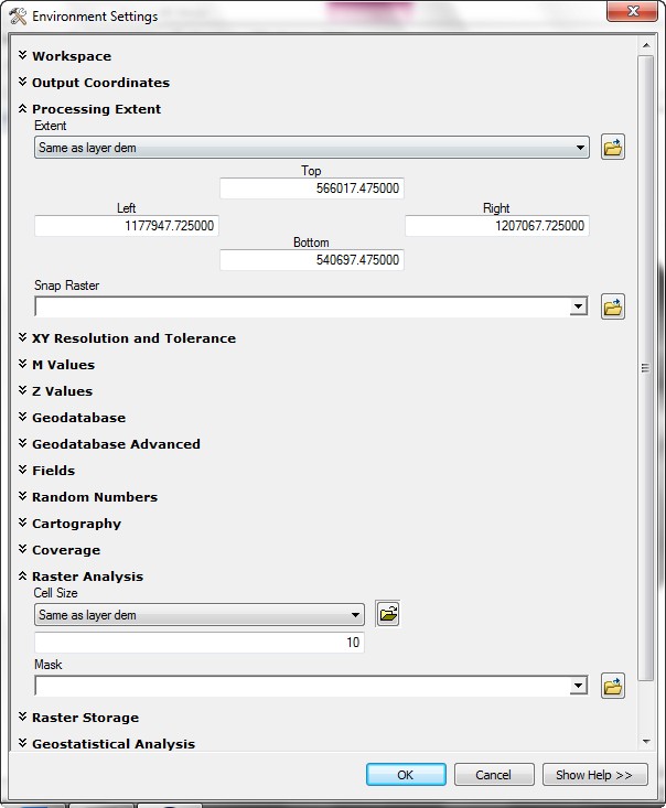
- Set the Geoprocessing > Environment > Raster Analysis and Cell Size to Same as layer dem. Also, open the "Processing Extent" tab and assign it as Same as layer dem.
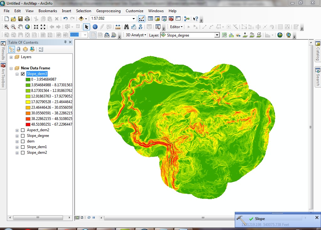
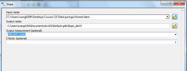
- Select Spatial Analysis > Surface > Slope from ArcToolbox.
- Areas that are green are less steep; areas that are yellow to red are steeper.
Create a percent slope grid
Percent slope is defined as (rise / run * 100%). Many professions use percent
slope for calculations rather than degree slope. The following image shows
how percent and degree slopes are defined:
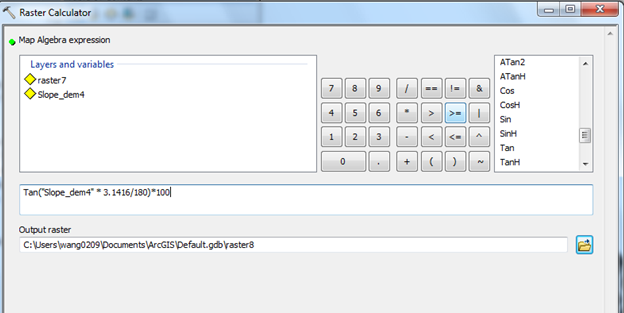
- From the Spatial Analyst menu, select Raster Calculator.
- Create a calculation to convert degree slope to percent (I suggest copy-and-paste
from the browser).
Tan("Slope of dem" * 3.1416 / 180 ) * 100
Question for the geometry geeks in the audience: What is the basis for
this conversion (why does it work)?
- Although the new grid looks the same as the original slope grid, the values
have been rescaled. Examine the values of the new grid. They should be in
a different range than the degree values.
- You can also do this the easy way:
Examining the cell values should show you that both methods of generating
percent slope result in the same data.
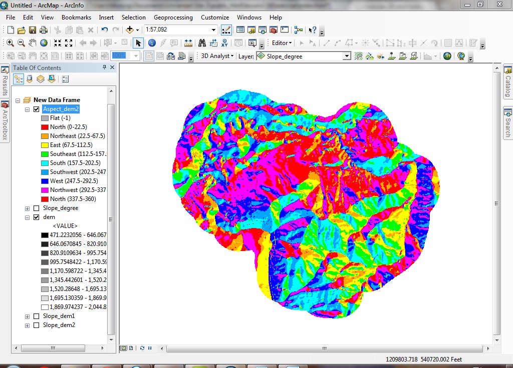
Create an aspect grid
- From the Spatial Analyst toolbox, select Surface > Aspect.
- The Aspect grid is symbolized with the same color scheme as the TIN. Looking at the same area as before, you can see how the aspect grid agrees
with the TIN.
Slope and aspect are often used for vegetation and habitat modeling. They are
also used for all types of other land-use planning, management, and development
regulations.
Find steepest descent path
Finding the steepest descent path shows the direction water will flow from
a user-selected location until slope levels off.
- Alter the default line symbol to make the default line symbol a thick magenta
line (in order to see descent pathways easier). All subsequent added graphical
lines will use this symbol. From the Draw menu, click on the Drawing tab, and select Default Symbol Properties.

Click the line symbol.
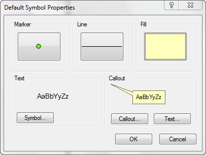
Select a magenta color and alter the thickness to 2 pixels and click on OK to finish this set up:
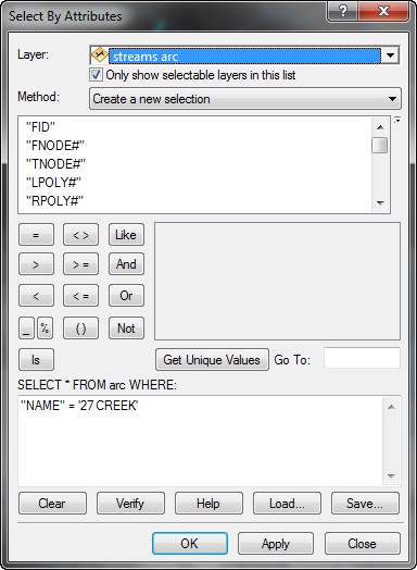
- Add the Streams layer into ArcMap, and zoom in to the 27 Creek area (north-central
Pack Forest, use Select by attribute to find out where this area is).
- Make sure the Layer in the 3D
Analyst toolbar is pf_tin.
- Click the Steepest Path tool
 .
.
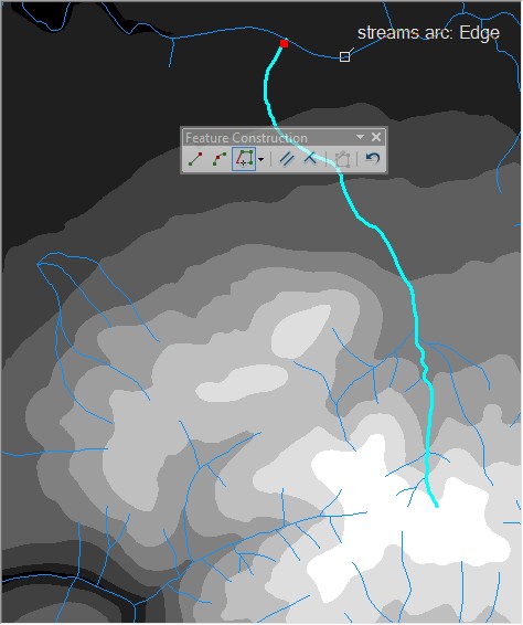
- Click the headwater as indicated in the image below. Notice how an anomaly
in the TIN causes the stream to jump from 27 Creek to the Little Mashel. Also
notice that the lines are added as simple graphics rather than as feature
layers. However, the lines can be converted to features later. These
"simple" graphics also contain 3D information (Z value on the vertices).
Note how the steepest path "jumps" from one stream to another. You may recognize
this surface model error later during the exercise on hydrologic modeling. [If you click at a location that does not flow downhill, use the pointer tool to the right of "Drawing" in the bottom toolbar, right-click on the selected box, and select "cut". This will can remove the magenta line.]
- Click again at the lower end of the first line to create another downstream
line. Continue the process until the line goes off the display extent.
- Select all graphics (from the Edit menu, choose Select All Elements).
- To create a new data set from the graphics, from the Drawing menu, select Convert Graphics to Features, creating the shapefile M:\3d\27_creek_3d.shp.
- To make the new layer clearly visible, delete all the graphics from the
data frame (Edit > Select All Elements then Edit > Delete).
This example finds the steepest downward path for water flowing to or in a
stream. Note that it has problems where flow pathways are not clearly defined in the surface data.
Similar analyses can be used to determine lowest-cost pathways for surfaces
that represent features other than elevation. Can you think of any other applications
for this analysis technique, using grid data other than elevation?
Analyze line of sight and create surface profiles
This process will allow you to analyze what parts of the landscape are visible
along a line of sight between an observer and a target. It allows you to
determine if an object or part of the landscape that is between an observer and
target can be seen.
- Make sure the dem layer is selected
in the 3D Analyst toolbar.
- Alter the symbology of the dem layer
so you can clearly see where ridgetops are (in my example below, there are
15 classes).
- Click the Create line of Sight
 tool on the 3D Analyst toolbar.
- Set the Observer offset to 6 ft
(roughly the height of an observer). Z unit here will be based on the projection unit.
- Click the observer location at the crest of a hill.
- Click the target across the Mashel River.
You can see where the landscape is visible (green) and not visible (red) along
the line of sight.
- It is also possible to get a surface profile, but not using the line of
sight (the sightline is not a 3D graphic). Instead, use the Interpolate
Line tool
 to create a 3D graphic. Trace over the sightline.
- Now that you have a 3D graphic, click the Create Profile Graph
 button. A graph will open that
shows the profile of the DEM along the sightline.
button. A graph will open that
shows the profile of the DEM along the sightline.
You have just created a line of sight between two points. This also includes
the functionality to create cross-sectional surface profiles, which is probably
more useful than just line of sight.
Create a viewshed
Viewsheds are similar to line-of-sight analyses, but are calculated on a landscape
basis rather than on a single line. These kinds of analyses are used in any kind
of research or planning where knowing the areas visible from a single location
is important (e.g., some kinds of wildlife studies, forest operations, cellular
phone tower locations).
- Zoom out to full extent.
- Create a new point feature class called M:\NetID.gdb\vis_point.
- Add a single point to the shapefile (Start Editing, use the Sketch
Tool) somewhere within the bounds of the surface models. (Your point can
be anywhere, not necessarily at the place I chose, though your viewshed will be more interesting if your viewpoint is placed at a high spot).
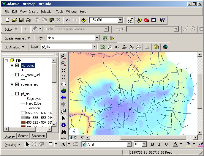
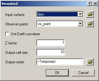
- From the Arctoolbox > 3D Analyst > Raster Surface, select Viewshed.
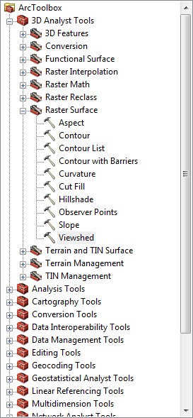
- Set the Input Surface to dem, Observer Points to the point layer you just created. Keep all other default settings. Remember, Z factor here does not mean the unit (like feet) but how many times of the origianl Z values
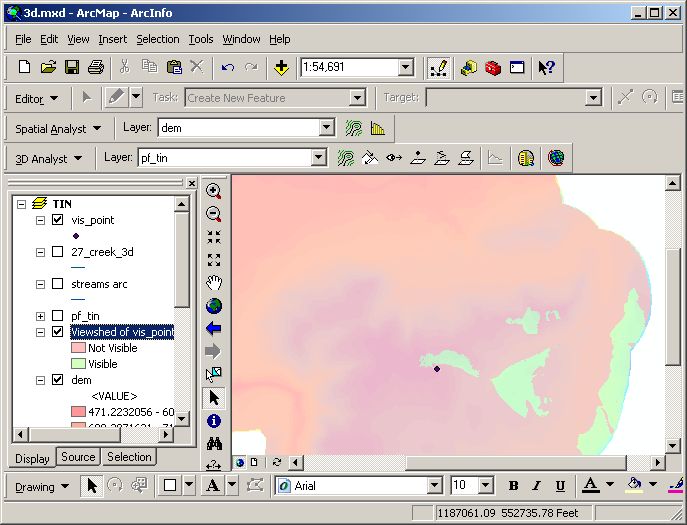
- Eventually a new grid will be added to the data frame, which shows areas
visible and not visible from the observer point. Remember that it is likely
your viewshed will look different from mine because it is unlikely your observer
point was identical to mine.
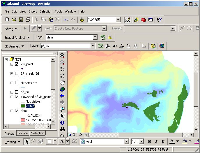
- Change the symbology of the output grid to better see where the visible
areas are.
Certain planning and management objectives need to consider visual impact of
activities. It is possible to generate the areas visible from a single point
or a number of points (for example, you could place points along a highway to
determine what parts of the landscape are visible from the road).
Create surface profiles from line features
- Open a new data frame.
- Add the streams and boundary layers to the data frame.
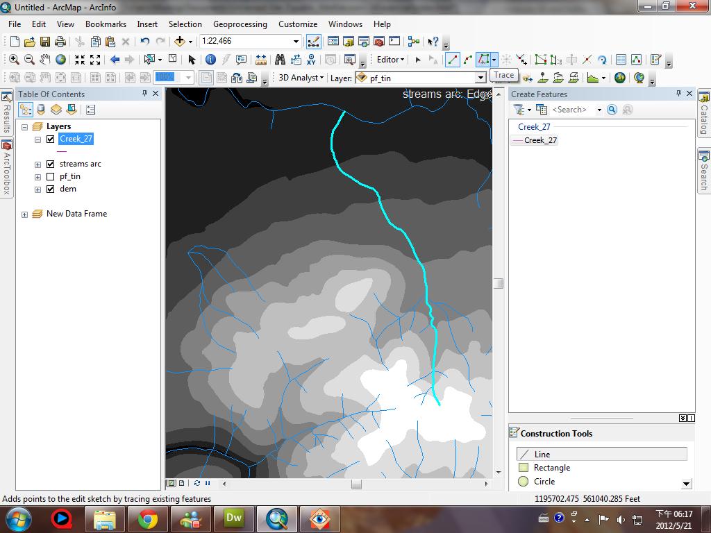
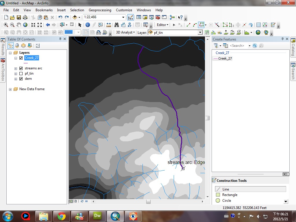
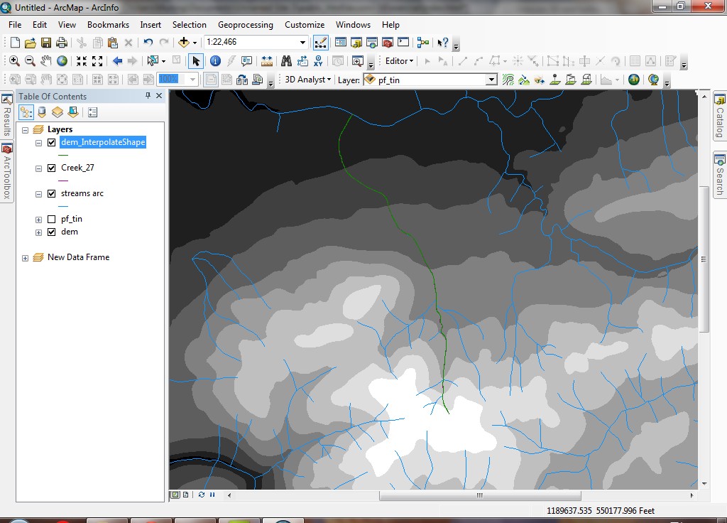
- Select the main stem of 27 Creek, as shown below:
- Create a new feature class called Creek_27
and add it to the data frame and select the one of the feature of Pack Forest (L:/packgis/forest) to import "Spatial Reference".
- Start editing.
- Use the Trace tool
to create a new feature in the Creek_27 feature class
that is spatially coincident with the selected features from the streams
data set.
- In order to store this as a 3D shape, it is necessary to convert it to
a new shapefile.
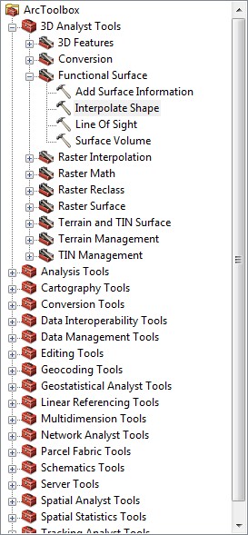
- From the 3D Analyst of ArcToolbox, select
Functional Surface > Interpolate Shape
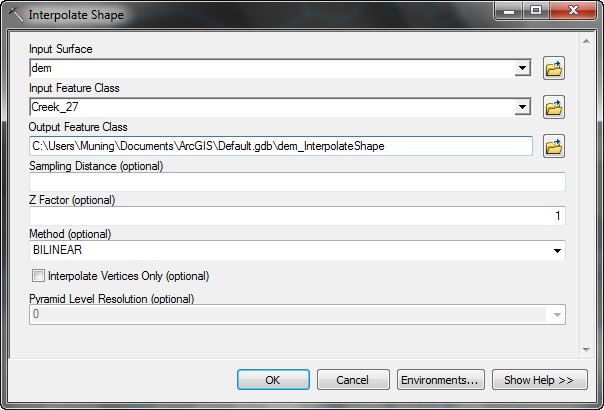
- Make sure to use the correct input data set. Take the Z values from the
dem grid.
- Put the output data in M:\NetID.gdb\dem_InterpolateShape.
- After the conversion is complete, add the data set to your data frame.
- Select the line that represents the main channel of 27 Creek.
Note: If you don't select the line, you can't activate the Create Profile Graph button below.
- Click the Create Profile Graph
tool. You now have a graph that shows the elevational change along the
stream line.
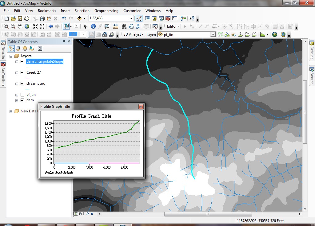
In the previous surface cross section, the line defining the cross section
was defined planimetrically as a straight line drawn between two points. In
this case, the surface cross section line is defined planimetrically as a curved
line (the flow path of 27 Creek). This functionality allows you to see
the surface elevation at various places along a curved line, such as a road
or stream.
Display landscape data in 3D
- Open ArcScene (from the same place on the Taskbar where ArcMap is started).
- Add the grid layer dem.
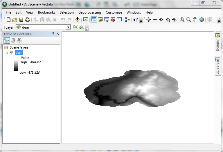
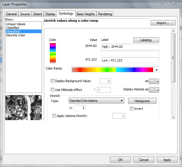
- Open the properties for the layer
- Alter the symbology to use a color ramp
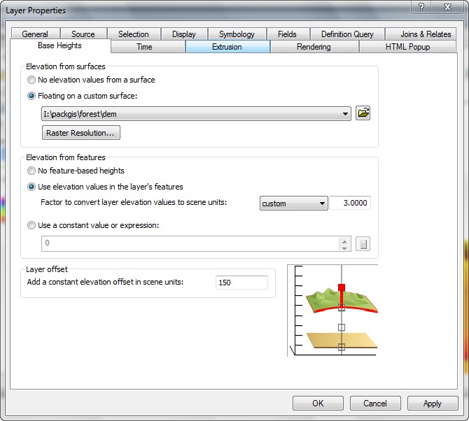
- Click the Base Heights tab.
- Click Obtain heights for... and make sure this is set to
the dem grid.
- Set a Z Unit Conversion of 3. This sets a vertical
exaggeration factor of 3.
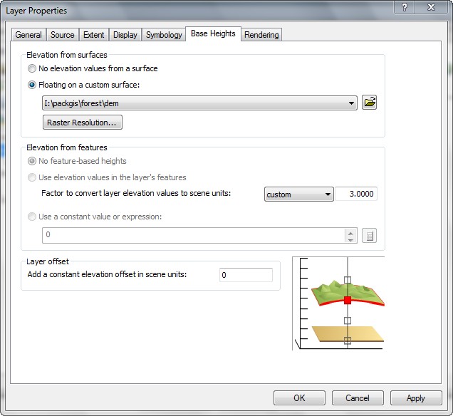
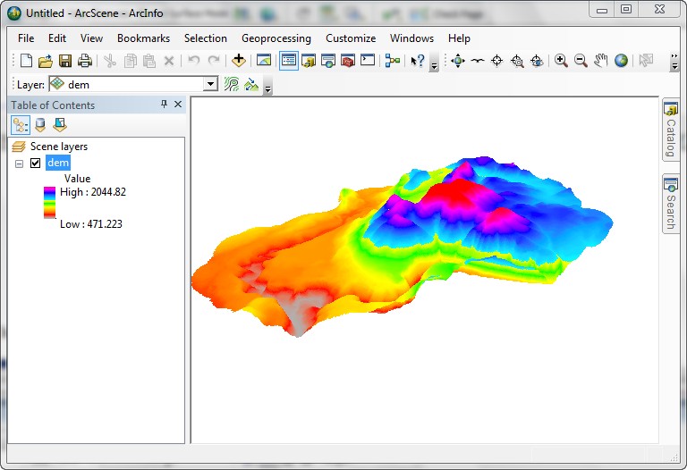
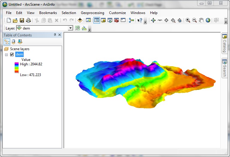
- Click OK. You will see a 3D display. Note it is difficult
to visualize the landform, especially in the mid elevations
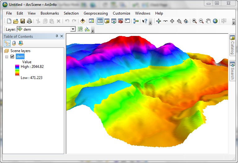
- Check Rendering > Shade areal features.... to apply an analytical
hillshade to the model.
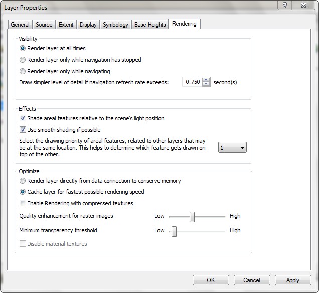
- Now you see the landform looks more realistic.
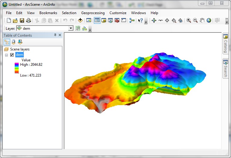
- Using the left mouse button, spin and tilt the surface model by moving
the mouse around.
- Using the right mouse button, zoom in and out by moving the mouse forward
and backward on the pad.
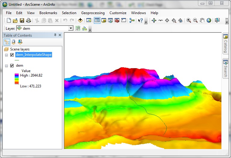
- Add the feature class we just created: dem_InterpolateShape.
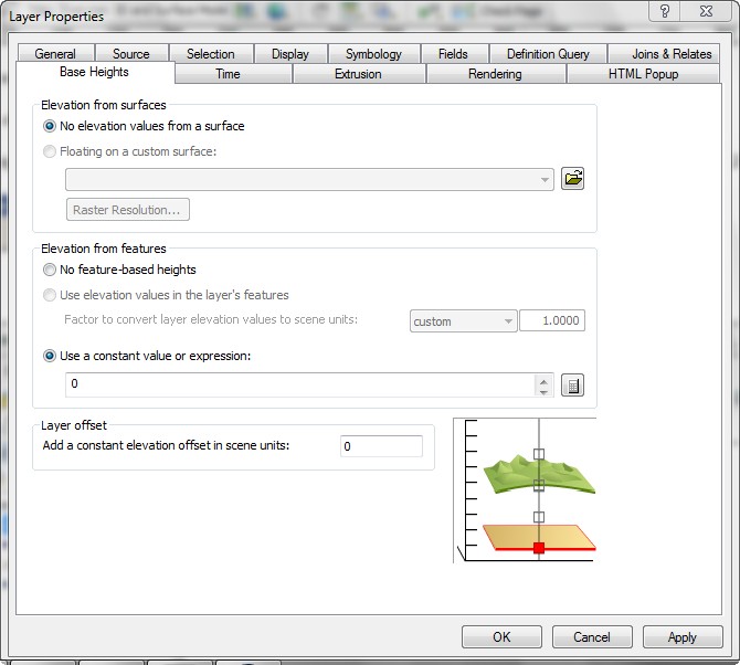
- Alter its Base Heights.
- Choose dem layer as the Elevation surface.
- Alter the Z Unit Conversion to 3.
- Add an offset of 150 to make the line stand above the surface.
- Navigate to the location of the 27 Creek 3D shapefile.
Display other (non-elevational) data in 3D
- Save the scene.
- Create a new scene.
- Add two copies of the cfi (plot centers) layer from the L:\packgis\forest
directory.
- Alter the base heights of the topmost layer so that the elevation of those marker points will
be conifer volume / 20.
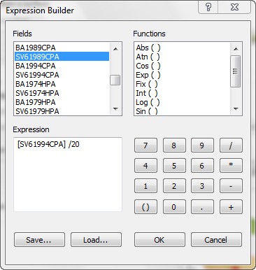
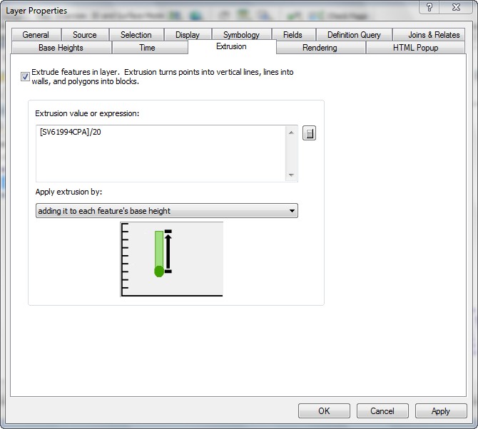
- Alter the second CFI layer 3D properties so that the markers will be extruded
by the value equal to the conifer volume / 20. The two CFI layers will create
a composite 3D marker (one layer as "poles" and the other layer as knobs at
the ends of the poles).
- Add the stands from the CD. Alter its symbology to show stand ages.
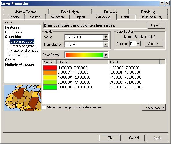
- Do you see any patterns here that you can explain?
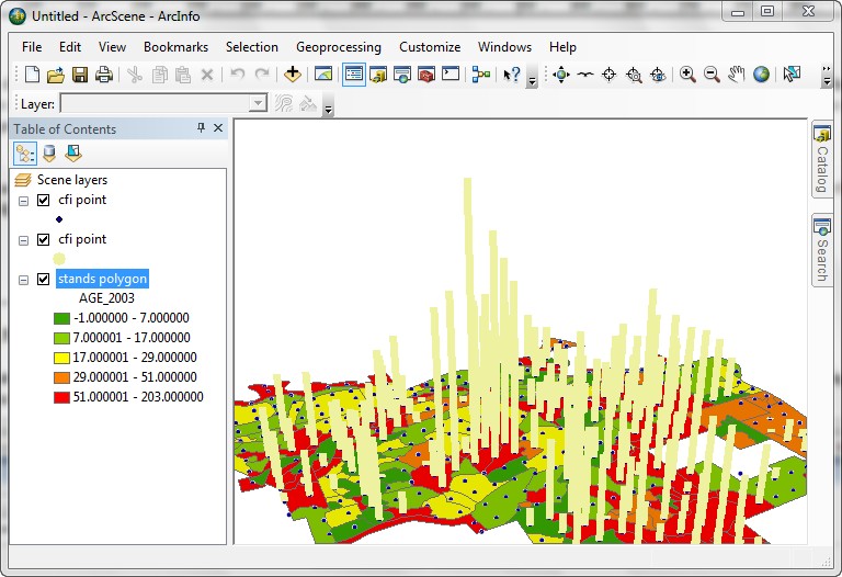
This displays a numeric attribute of CFI plots as a 3D value. It is easy to
see the location of plot centers with the greatest conifer volume, and where
these are in relation to stands. The data we are viewing have nothing to do
with elevation, but applying 3D display makes the data in some ways more comprehensible.
Displaying non-elevation data in 3 dimensions is a technique that can be used
to communicate values without needing any explanation other than the image and
the knowledge of the variable being displayed. What other kinds of data can
you think of to use in 3D display?
REMEMBER TO TAKE YOUR CD AND REMOVABLE DRIVE
WITH YOU!!!!
Return to top
 |
|
TThe University of Washington Spatial Technology, GIS, and Remote Sensing
Page is supported by the School of Forest Resources
|
|
School of Forest Resources
|
 UW
Home
UW
Home