
Introduction to Geographic Information
Systems in Forest Resources |
Exercise: Watershed
Delineation
Objective:
- to learn how to use surface hydrologic modeling tools in ArcGIS
- Perform drive
substitution to create drives L (CD) and M (removable drive).
- Start ArcGIS and create a new map document
- Watershed Delineation
- Creating a depressionless DEM
- Flow direction
- Flow accumulation
- Create watershed pour points
- Delineating watersheds
- Automatically delineating watersheds ("Basins")
- Calculating flow length
- Raster to vector conversion (stream network as
line shape)
- Watershed visualization
Perform drive substitution
Perform drive
substitution to create the virtual drives L and M.
Start ArcGIS and open a new map document
- Delete everything from your removable drive.
- Create a directory on the hard drive (I suggest C:\Users\NetID\Document\ArcGIS). This
will be used to store files temporarily.
- Create a directory (M:\hydro). If you create a directory by a different
name, make sure to be consistent. If you create a directory that has spaces
anywhere in the pathname, expect things not to work properly.
- Open ArcMap.
- Enable the Spatial Analyst Extension (Customize > Extensions...).
- Add the layer L:\packgis\forest\dem to the data frame.
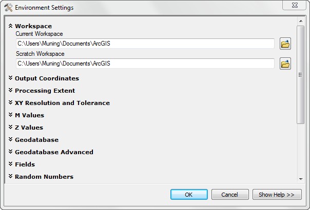
- Set some environment properties (Geoprocessing
> Environments)
- Set the Current Workspace, Scratch Workspace, and Output
Extent as below:
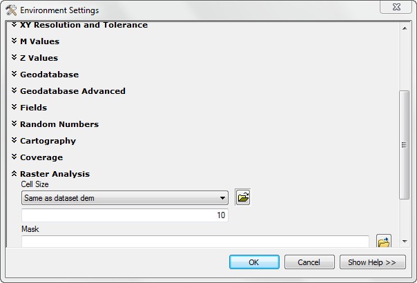
- Set the Cell Size as below.
- Save the map document as M:\hydro\watershed.mxd.
Watershed Delineation
Creating a depressionless DEM
It is important to start with an elevation grid that has no depressions.
- Open the ArcToolbox toolset Spatial Analyst Tools > Hydrology.
This is where the surface hydrology tools are located.
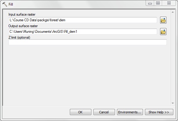
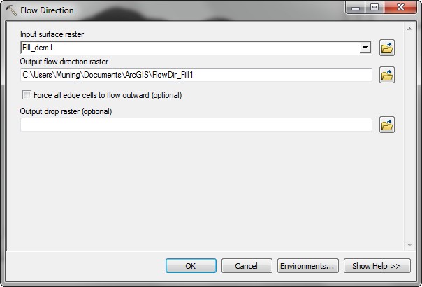
- Open the Fill tool. The input surface is the dem grid. Output
is C:\Users\NetID\Document\ArcGIS\Fill_dem1 (the default name).
While the grid is filling, which may take a few minutes, you might want to
entertain yourself with the
Onion.
- After a few minutes, a new layer, fill_dem1, will be added to the
data frame.
This is identical to the dem raster, but any areas of internal drainage
are filled in.
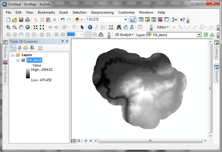
Note the difference in the lowest elevation value in the legend; sink cells
in the original data set have been filled in.
- Delete the dem layer from the data frame, since you will be working
on the filled grid from this point on.
It is important to have a depressionless DEM for all subsequent hydrological
analyses. Areas of internal drainage can cause problems later in the watershed
delineation process.
Flow direction
- Open the Flow Direction tool.
- The input surface is the Fill_dem1 grid.
- The output raster should be set to C:\Users\NetID\Document\ArcGIS\FlowDir_fill1
(the default)
- Turn off display of the Filled dem layer.
- Add the layer L:\packgis\forest\streams to the data frame You should
start to see some patterns.
- Note that the numbers refer to coded
direction of flow.
Direction of flow must be known for each cell, because it is direction of
flow that determines the ultimate destination of water flowing across the
surface.
Flow accumulation
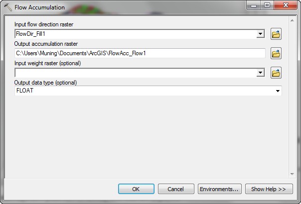
- Open the Flow Accumulation tool.
- Set the input flow direction raster (FlowDir_fill1) to the output of the last task.
- Set the output raster to C:\Users\NetID\Document\ArcGIS\FlowAcc_flow1 (default
name).
- Turn off the Flow Direction layer. The flow accumulation layer has
a value for each cell; that value represents the number of cells upstream
from that cell. Cells with higher values will tend to be located in drainage
channels rather than on hillsides or ridges.
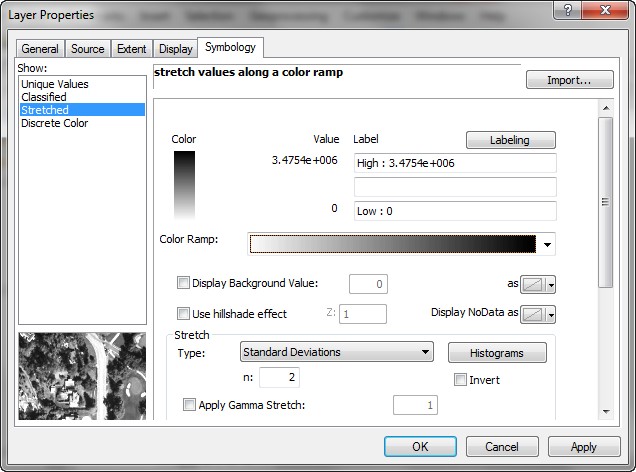
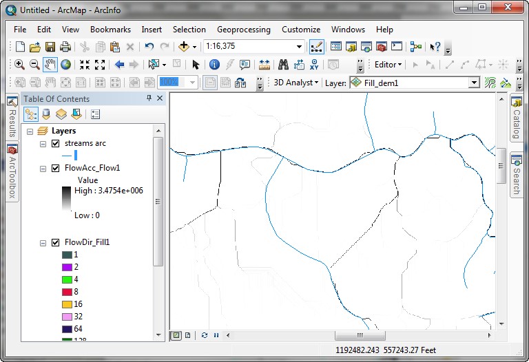
- In order to make each flow is visable, you need to modify the symbology to make it work. If you are in the MGH lab, since the map server is done and can not be fixed so far, if you can not run the "Symbology" to classify, you need to reverse the color ramp in the symbology -> Stretched tab. Adjust your color ramp from WHITE to BLACK, as the following snapshot.
- If you are working this in the Suzzallo Lib or your own computer, please follow the following steps:
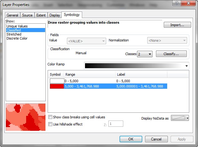
alter the legend for this layer. It will be easier to visualize high-flow
pathways by altering how cells are displayed.
- Change the symbology method to classified. Use 2 classes.
- Alter the break value for the first class to 5000.
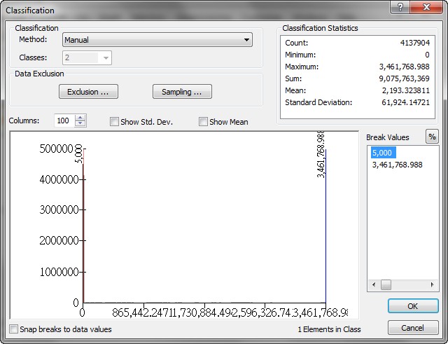
- Change the symbology (no color for the first class, red for the second
class).
Now the cells that are displayed in red have the flow of at least 5000
upstream cells flowing through them. This translates to an upstream area
of 11.5 acres. 5000 cells * (100 ft^2 / cell) * (1 ac / 43560 ft^2) =
11.5 ac.
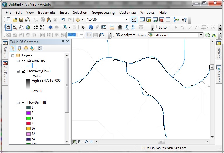
You should also see that the DEM-generated drainage network looks somewhat
like the vector streams, although if you look at details you will see
where the data sets do not line up.
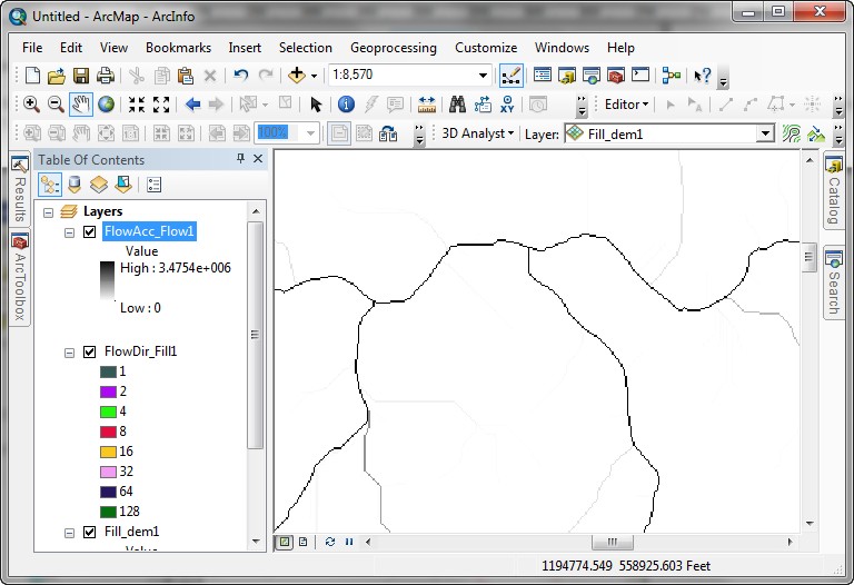
You will need to zoom in before you can see the details of the flow network.
Flow accumulations are important because they allow us to locate cells with
high cumulative flow. Pour points must be located in cells of high
cumulative flow, or the resultant watersheds will be very small.
- Use ArcCatalog now to copy the fill, flow direction, and flow
accumulation grids to M:\hydro (this will require about 65 MB of
space).
Create watershed outlet ("pour")
points
- Create a new point shapefile in ArcCatalog (M:\hydro\pour_points;
copy the coordinate system parameters from one of the other Pack Forest data
sets).
- Add the point layer to your map document.
- Download this zipped generate file (pour.zip) which has two boxes indicating the location to create pour points.
- Add the new point layer to your data frame and begin editing (edit the folder that contains the point data set you created in step 1).
- In order to see better where you are adding points, open a magnifier window
(Window > Magnifier).
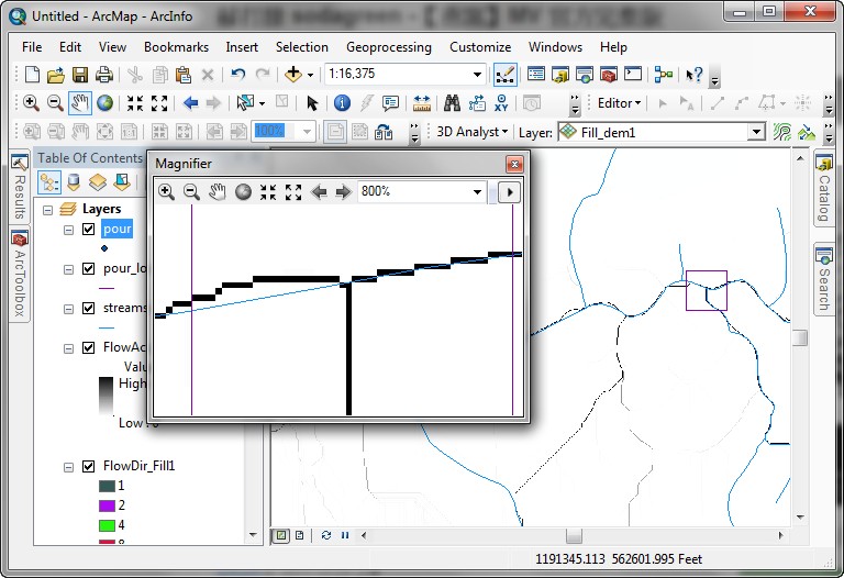
- You may need to zoom in and increase the zoom factor of the magnifier (right-click
the magnifier's title bar and select Properties) before adding any
points.
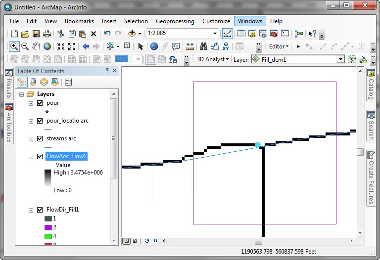
- Use the Identify tool to examine the values of the Flow Accumulation
layer before adding any points. You will be able to tell which direction the stream is flowing by looking at the elevations of a number of identified points. Upstream locations will have lower accumulation value and downstream will have higher
accumulation value (why is this?).
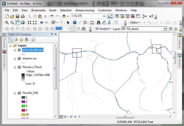
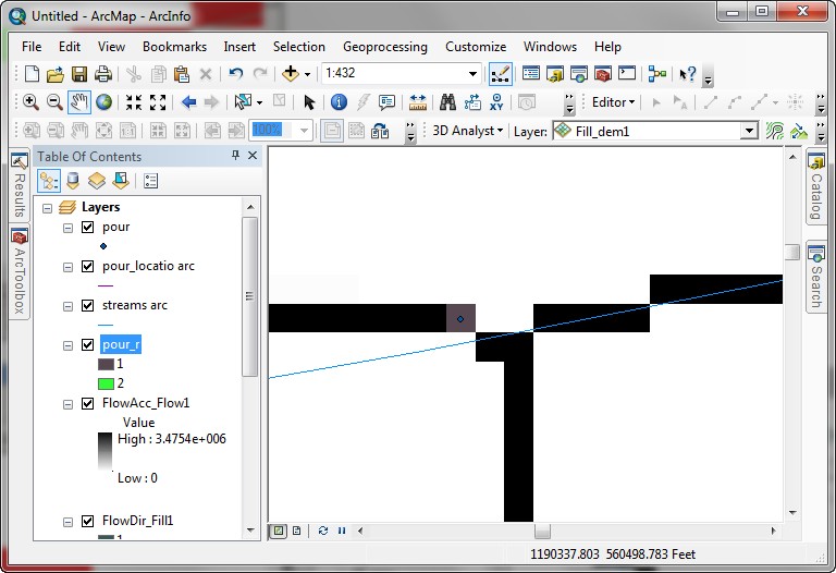
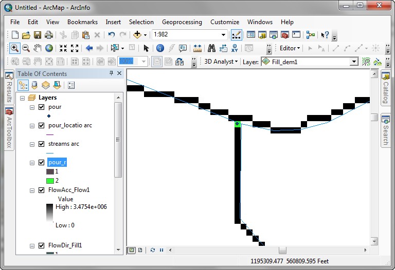
- Start editing (make sure you specify the correct folder to edit). Add points at high-flow locations. Refer to the images below for more precise placement.
Western point: note the position of 27 Creek (the stream network in the center
of this image of the data frame). The watershed we are creating is just west
of 27 Creek's confluence with the Mashel River. At that location, there is
no stream in the vector data.
Eastern point: this watershed (Little Mashel) is east of 27 Creek. The pour
point is upstream of the confluence on the Little Mashel River.
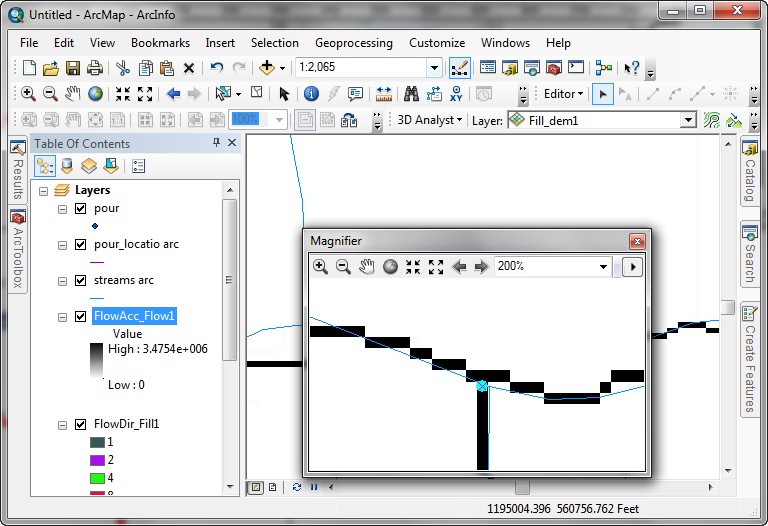
| You must
zoom in quite a way to do this, otherwise your pour point may not
be located within a high-flow pathway!
If your points are not in a high-flow pathway, move them before proceeding. |
Everything upstream from each one of these points will define a single watershed.
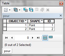
- Open the attribute table for the pour_points layer. Alter the ID
field to represent unique values for each different record (e.g., 1
and 2). Watersheds are defined by
pour point IDs; if you do not alter the ID values for the points, there will
be only one value, and you will not generate unique watershed areas.
- Once you have added the points and altered their IDs, stop
editing the layer, making sure to save the edits.
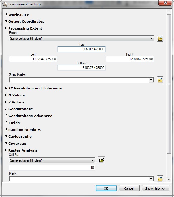
- Select Geoprocessing > Environments > Processing Extent to make sure the output extent the same as the filled DEM (fill_dem1) so the extent will be correct
(you don't want the watershed truncated). Also set the cell size in Raster Analysis.
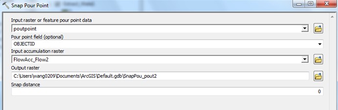
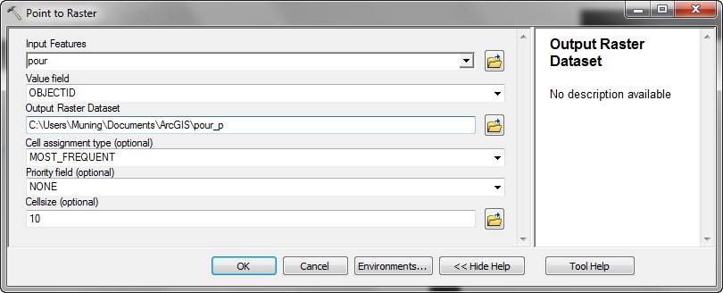
- The watersheds are not generated directly from point features, but by raster
cells. In order to convert the points to a grid, use the tool Spatial Analyst Tools> Hydrology > Snap Pour Point or Conversion Tools>To Raster>Point to Raster
Alter the drawing order so you can see all the layers clearly. Zoom
in as needed to verify that the new cells overlap with the high-flow pathway.
If the Analysis Extent and cell size do not match an existing layer, there
may be problems of registration between the pour grid and the other grids
necessary to delineate watersheds. Therefore, it is always a good idea
to set your cell size and analysis extent relative to an existing grid
layer.
Note that the new feature_pour1 layer cell covers the place where
the last pour point was added. If the pour grid cells are not in high-flow
pathways, the watersheds you create will be small. If the pour grid cells
are not directly "over" the flow path, you will not create watersheds
that represent large drainage areas.
Delineating watersheds
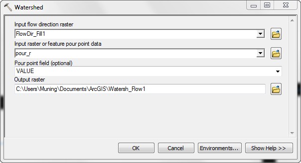
- Open the Watershed tool. Note that one of the options for the input
data (as shown below) is the point feature dataset (pour_points). DO NOT USE THE POINTS!! Selecting a point
feature dataset will work in theory, but there is no way to verify your point features
will fall in a high-flow pathway. That is the reason for the conversion to
raster in the previous step. It is recommended to have converted the points to
a grid first, which verifies that the pour point locations are in the high-flow
pathway.
- Select the flow direction grid as the input flow direction raster.
- Select the raster version of the pour points as the input raster.
- Accept the other defaults.
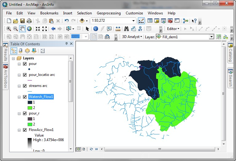
- The new watershed grid will be added to the data frame.
These two large grid zones represent the areas upstream from the selected
pour points. The western pour point defines the entire watershed system (both
grid zones). The basin to the south and east is really a sub-basin of the
larger system. Its pour point is upstream of the western pour point.
- You can verify this by altering the drawing order and zooming into the
upstream pour point. Note how the sub-basin contains the drainage network
for its sub-basin. Remember this pour point was selected to be upstream of
the confluence.
You have just delineated two watersheds, based on your elevation grid data
and the pour points you chose. If your watersheds are very small, it is because
you located your pour points outside of a high-flow pathway, or you did not
fill your original input elevation grid.
Automatically delineating watersheds
Compare your manual method with an automated method.
- Open the Basin tool.
- Select the previously created flow direction grid.
The automatically delineated watersheds are defined by pour points at
the edge of the grid.
- Convert these to polygons as well in order to see where the watershed
boundaries are. Make sure to uncheck Simplify polygons in order
to match the actual grid zone boundaries rather than generalizing lines
in the output.
- Zoom to the northwest of the grid. You can see a number of very small
basins.
- Open the attribute table for the new polygon data set. There are 413
basins.
You have just let ArcGIS automatically generate a series of watersheds. Automatic
watershed delineation is easy, but does not give you the control to create basins
specifically for pour points of your own selection. For this reason, the manual
method is used almost exclusively.
Calculating flow length
Flow length shows the distance water will need to travel across the grid.
- Open the Flow Length tool.
- The input raster is the flow direction grid created earlier.
- Use defaults for the other controls.
- Alter the color ramp so you can see the differences between low flow length
and high flow length areas. In this color ramp, the red cells are at the upper
reaches of streams in the forest, and the blue cells are farther downstream.
This shows the flow length to the ultimate pour point for each cell. Suppose
you want the flow length to the closest downstream high-flow pathway, rather
than to the ultimate outlet. This is possible, using flow length with
a weighting grid.
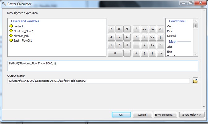
- Create the weight grid by making a grid whose values are no data
within the 5000-cell high-flow path, and values of 1 elsewhere. This is done
with a setnull function in the Raster Calculator:
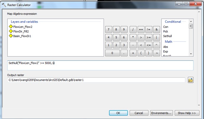
This calculation means:
"make a new grid; where the flow accumulation
cells have a value greater than or equal to 5000 in value, make those output
cells null; where the flow accumulation cells are less than 5000 in value,
make the output cells have a value of 1"
- Use the new grid as a weight grid in the flow length tool.
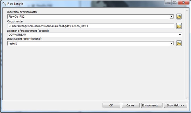
- The output grid now has values that represent the flowlength-distance to
the closest high-flow pathway rather than to the ultimate outlet.
Raster to vector conversion (stream network as line shape)
Raster data sets can represent drainage networks (e.g., the flow accumulation
cells that have at least 5000 upstream cells). When making maps that present the
results of watershed delineation you may want to show the grid-based flow network
instead of, or in addition to, the vector stream network, especially if the two
flow networks do not agree.
- First, create a grid that represents only high-flow (5000 +) cells. This
is also done in the Raster Calculator, similar to what was done in the last
step.
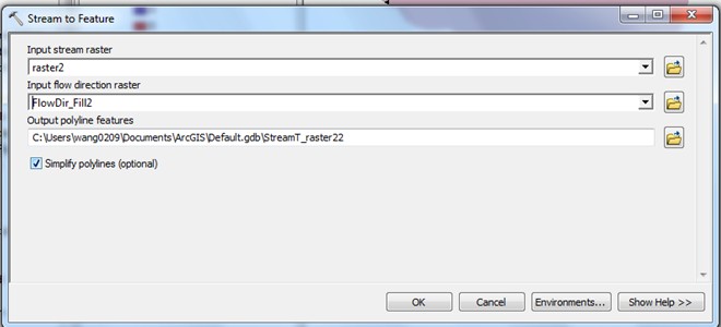
- Open the Stream to Feature tool.
- The input stream raster is the result of the last calculation.
- The input flow direction raster is the flow direction grid that was
made before.
Watershed visualization
The last step for this lesson will be to visualize the watersheds created earlier
with other data.
- Create a new data frame.
- Add a copy of the grid layer fill_dem1 from the other data frame.
- Create a hillshade grid from fill_dem1.
- Add the pour_points point feature layer.
- Add the line feature layers Contour and Streams from the CD.
- Add a copy of the watershed1.shp polygon feature layer.
- Alter its legend so that is is not filled and displayed with a red outline.
- Alter the drawing order and legends so that features are discernible. Does
this look reasonable to you?
- Visualizing in ArcScene can also be helpful.
REMEMBER TO TAKE YOUR CD AND REMOVABLE DRIVE
WITH YOU!!!!
Return to top
 |
|
The University of Washington Spatial Technology, GIS, and Remote Sensing
Page is supported by the School
of Forest Resources
|
|
School of Forest Resources
|
 UW
Home
UW
Home