Introduction to Geographic Information
Systems in Forest Resources |
Exercise: Raster
Analysis I
Objectives:
- to become familiar with raster data and simple raster analysis
- Perform drive
substitution to create drives L (CD) and M (removable drive).
- Clean out M:\
- Open an existing project
- Raster (grid) layer basic structure
- Change data (pixel) type: floating-point to integer type
- Alter the display of a raster grid layer
- Query a raster grid layer (Integer Type Only)
- View a histogram for cell value distribution
- Set analysis properties
- Raster Calculator (I): Perform a map query on a raster grid layer
- Raster Calculator (II): Perform a map calculation on a raster grid layer
- Raster Calculator (III): Querying across multiple grid layers
- Raster Calculator (IV): Conditional processing
Perform drive substitution
Perform drive
substitution to create the virtual drives L and M.
Clean out M:\
Because raster grid datasets take up a lot of space, you should delete any
unnecessary files from M:\. Delete everything from your removable
drive before starting the exercise. If you have been creating PDF files for
your assignments and saving them on M:\, these (as well as any old *.prn files)
can be deleted. If you need to save any data on M:\, zip and copy them to your
dante account or store them temporarily on the hard drive or write them to a
CD. If you run out of space during this exercise you may have problems....
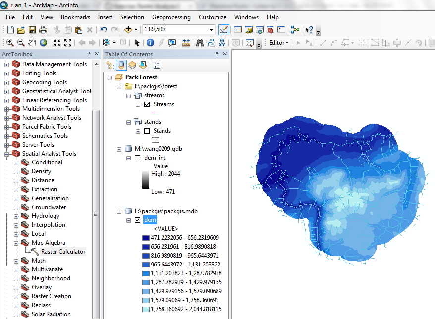
Open an existing project
- Download the project r_an_1.mxd, and save
it on M:\.
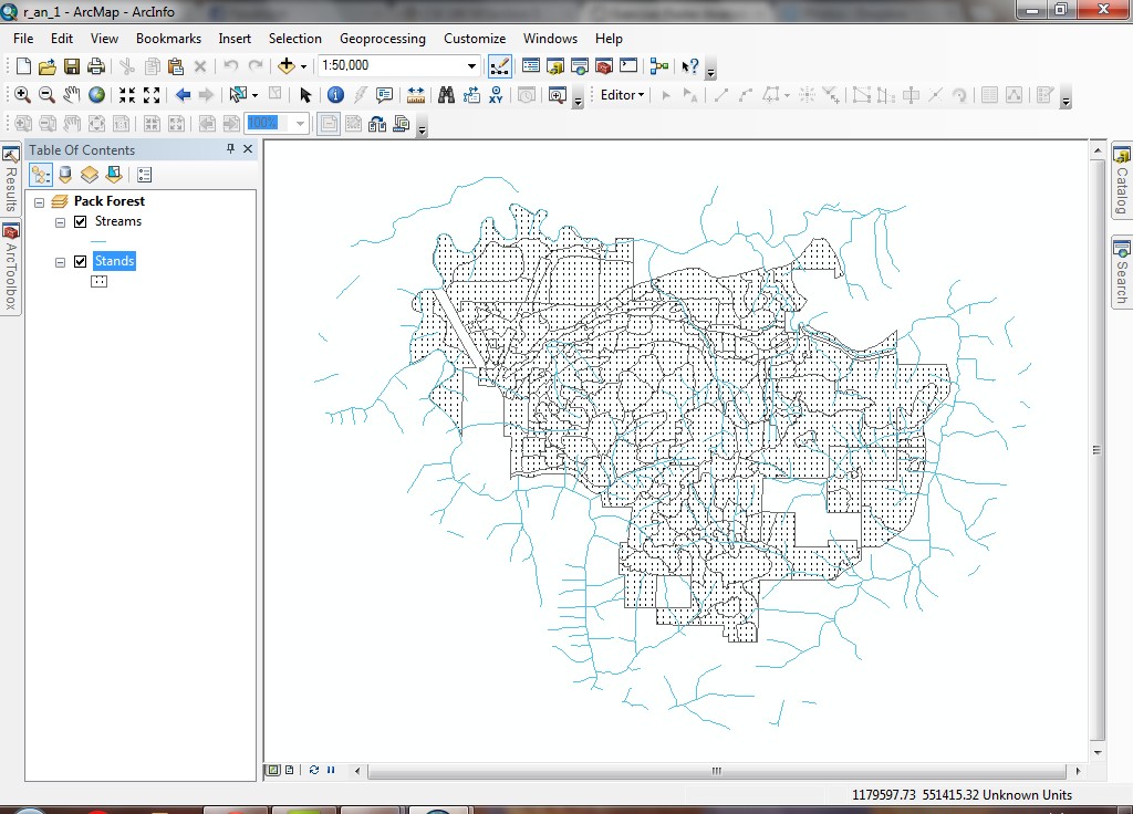
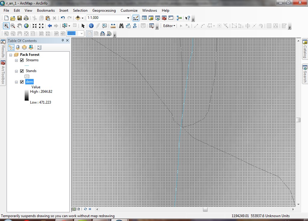
- When the project opens, it should contain the Pack Forest Stands
layer, as well as the Pack Forest Streams layer.
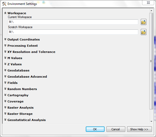
- Before doing anything else, set your Current Workspace to M:\
(Geoprocessing > Environments).
Raster (grid) layer basic structure
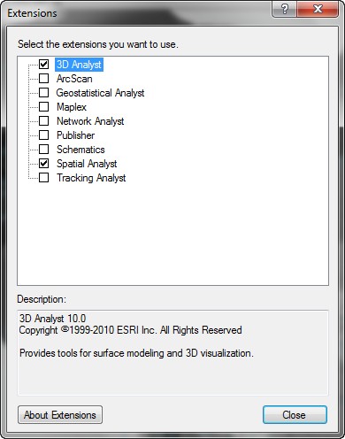
- In order to perform analyses with raster data, it is necessary to enable
the Spatial Analyst Extension and to display the Spatial Analyst Toolbar.
You can still add rasters to a data frame without the Spatial Analyst, but
they will behave only as simple images, and will lack analytical functionality.
- Select Customize > Extensions and click the checkbox for Spatial
Analyst.
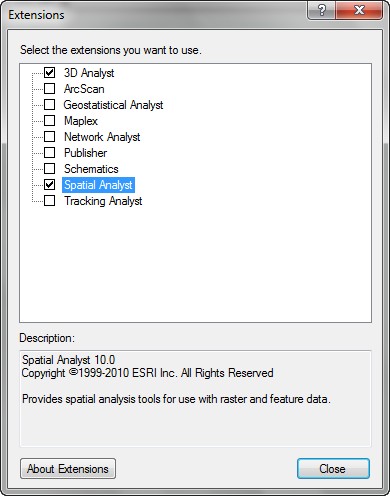
Click Close.
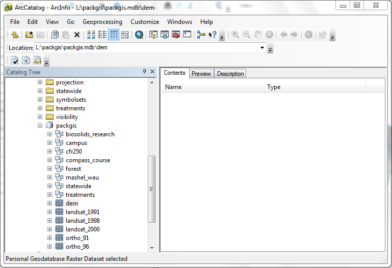
- Find L:\packgis\packgis.gdb\dem with ArcCatalog and look at its metadata.
Add this raster dataset dem to the data frame. Rasters are
added in the same way as any other data set.
- Make sure that Dem is the first (top) layer to draw, or it will obscure
your other data.
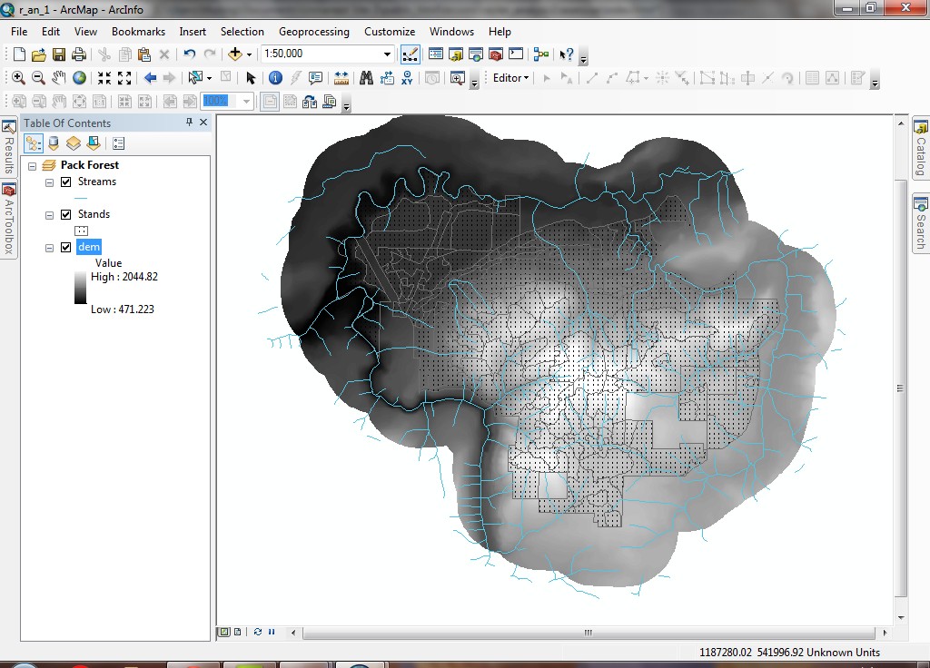
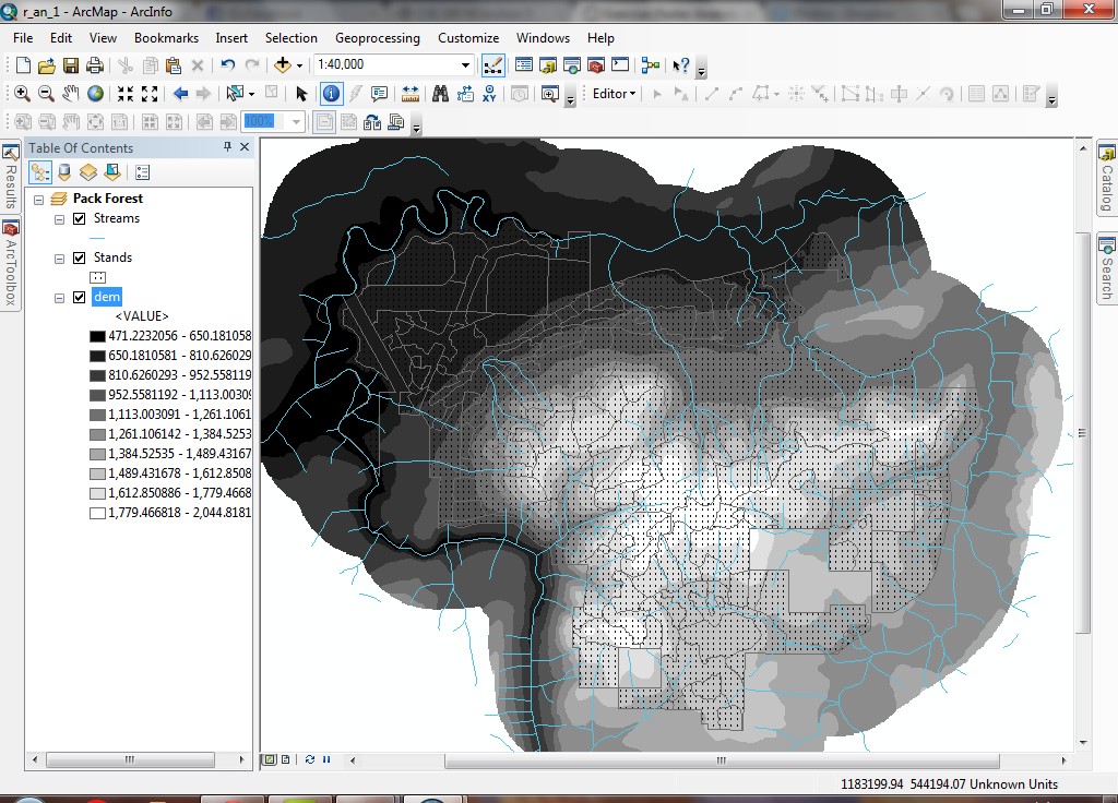
The raster dataset dem will be displayed with a greyscale stretched
Color Ramp. Note the values in the legend: these represent elevation in feet.
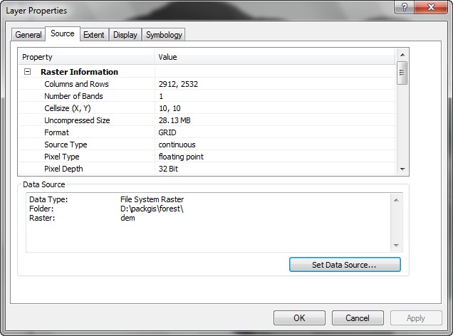
- Open the Properties for the layer. Click the Source tab. You
should always look at properties for layers, especially raster data, because,
unlike vector data, rasters have more properties that can affect your analyses.
Here, you can see the Cellsize (10 ft x 10 ft, the area of each cell is 100 ft^2).
Pixel Type is floating point (meaning decimal places can be
stored).
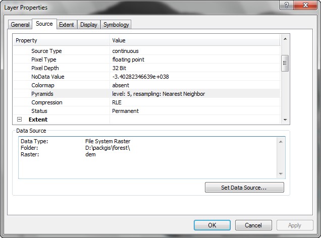
Pixel Depth is 32 Bit (floating-point values can range from
-3.402823466e+38 to 3.402823466e+38)
Pyramids are Present (with Level 5 and other status), which means the grid can be displayed
quickly at different zoom scales.
Many of the operations we will perform
will create temporary grids, which once removed from the map document, will
be deleted from the disk.
Close Properties.
- Zoom in until the map scale approaches 1000:
Note as you zoom in, you do not see individual cells. This is because the
Stretched symbology method also applies a resampling to smooth the
appearance of the display.
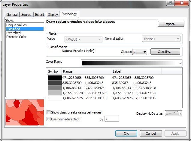
- Open the Properties for the layer and click the Symbology
tab.
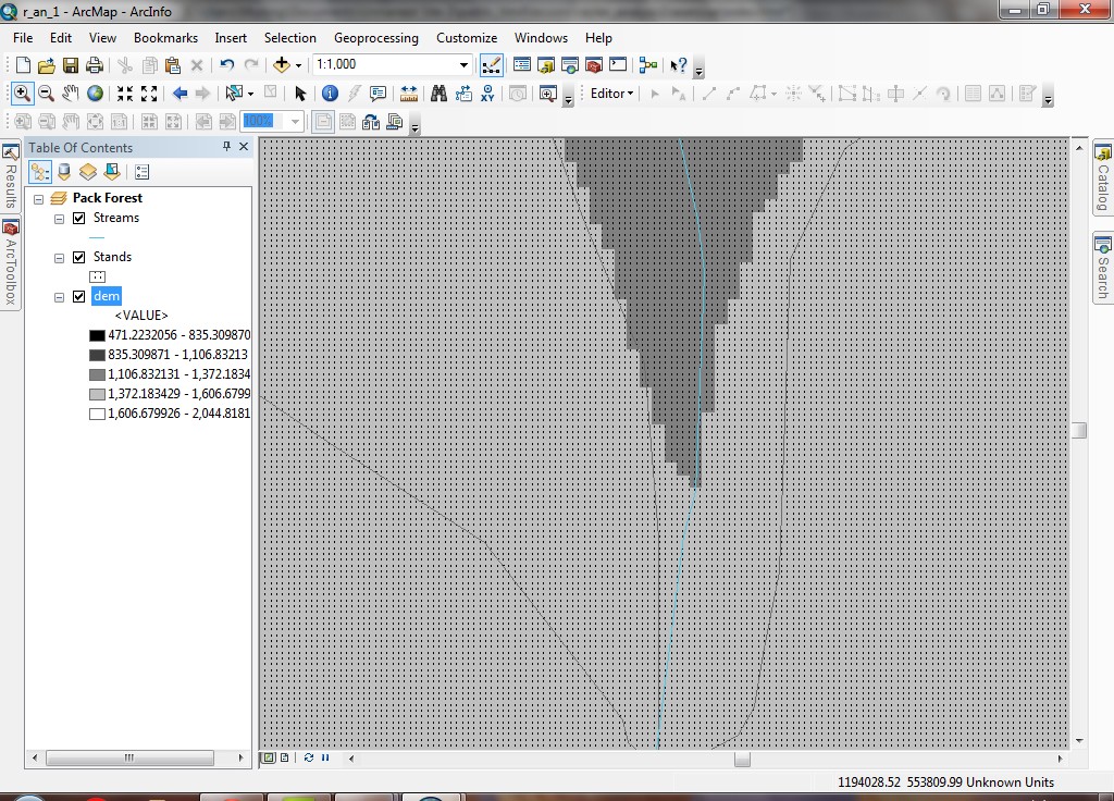
Click the Classified method. You will see the symbology changes to
a 5-class Natural Breaks classification. (MGH lab computer will not be able to perform this process, please read through it.)
- Now you can see individual cells. You may need to pan in order to see cells
at the edge of a class break.
- Turn off the Stands layer and with the Identify tool, click on a
few cells to see their elevation values. To view the results of multiple Identify
clicks, use the <SHIFT> key and click multiple locations. Note the values are floating-point
(that is, they have decimal place values).
.
You have just loaded a raster grid layer to a view. Make sure that you have
the Spatial Analyst extension loaded before you try to add raster grid
layers, or you will end up loading the image layer, which will be useless for
analysis.
Alter the display of a raster grid layer
When raster grid layers are loaded, they are loaded in 10 classes (9 numerical classes,
and 1 No Data class) with a random color ramp scheme. You may want to alter
the symbology for the display of different types of data.
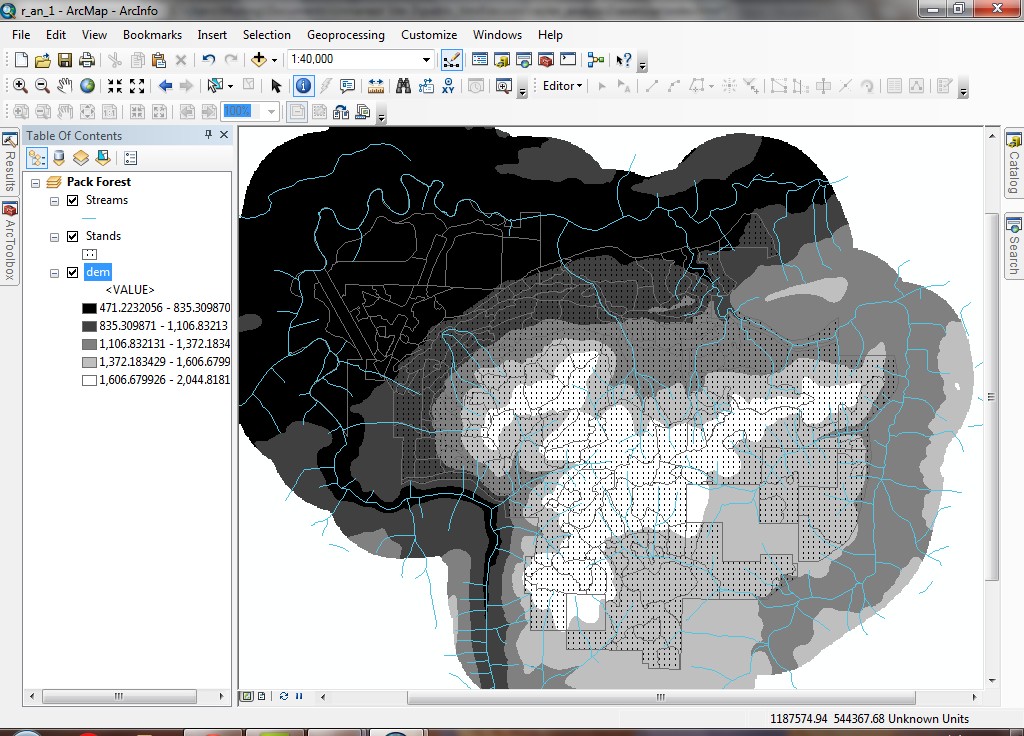
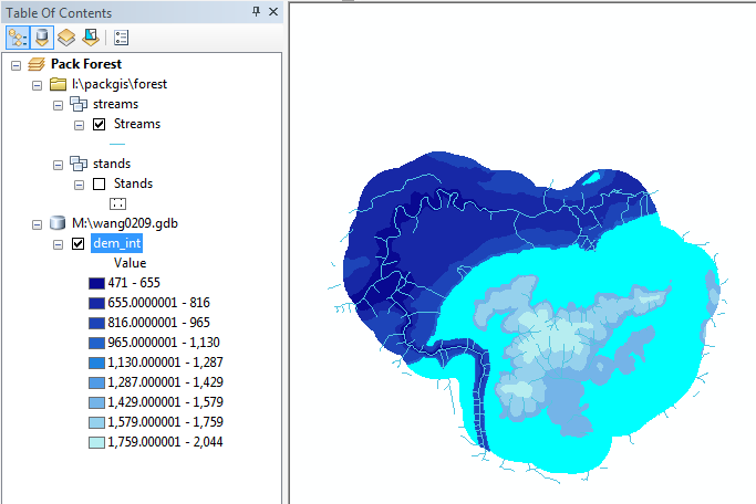
- Zoom back out to full extent. You can now clearly see the effect of the
classified display.
- Change the number of classes to 10 for a better display (MGH lab computer will not be able to perform this process, please read through it):
While the topography is becoming more apparent, it is still better to display
continuous data with a stretched, rather than classified, symbology.
- Open the layer Properties again.
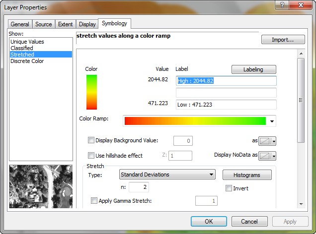
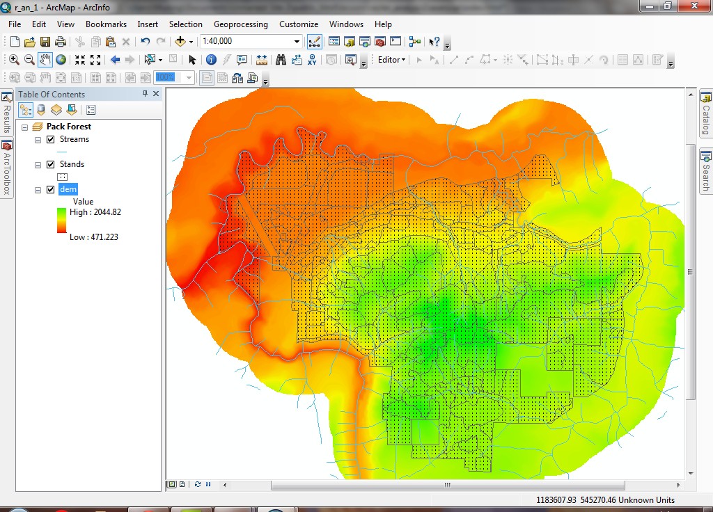
- Switch back to Stretched and select the Color Ramp that goes
from red to green.
- Click the Invert checkbox in order to have the colors go from
green to red with increasing elevation (the default method will display
lower elevations in red).
- Feel free to try a few different color ramps. Note that you can click
Apply in the Properties dialog to see the changes in symbology
rather than clicking OK. This will allow you to
choose different symbologies quickly.
- In order to see the numerical distribution of values you can set the legend
to Standard Deviation classification.
(MGH lab computer will not be able to perform this process, please read through it.)
- Open the layer properties > Symbology and select Classified.
Click the Classify button and choose the Standard Deviation
method.
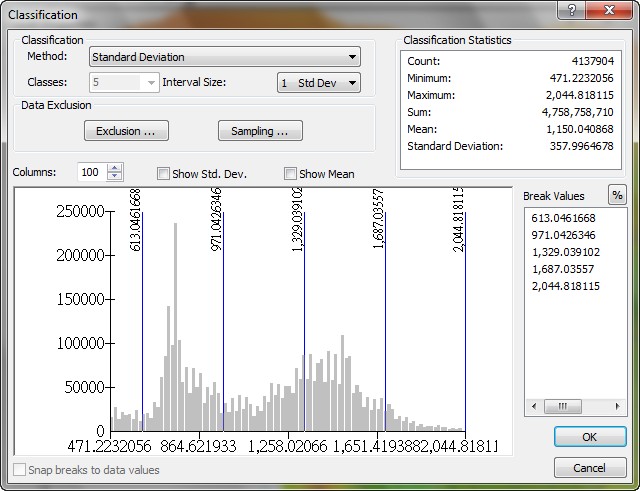
Note the mean elevation value for the data set is 1150 ft. The mean in
this case represents the quantity:
which translates to "sum all cell values and divide by the number
of cells."
Alter the Label for the classes as shown below:
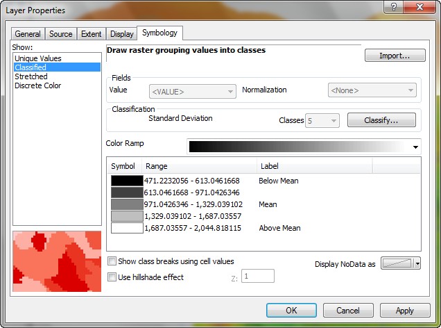
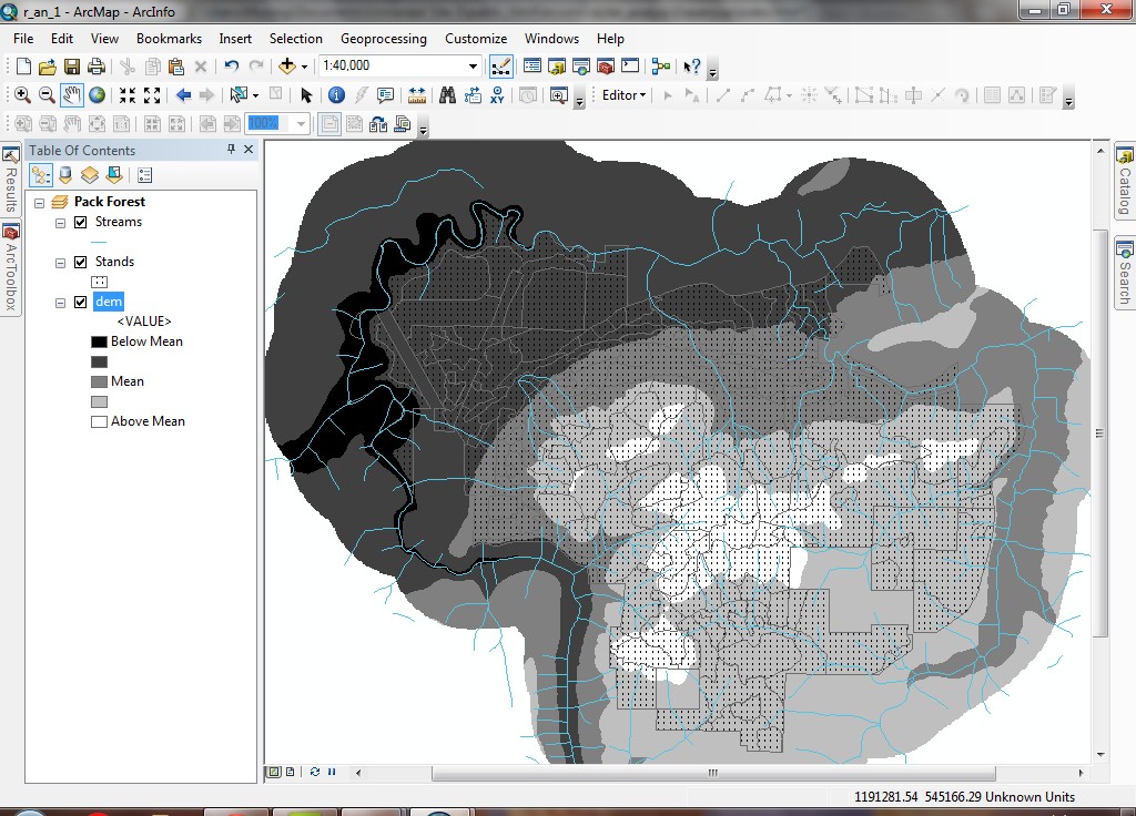
The legend gives you an idea of the statistical spread of your data, and
the view shows you the location of the different statistical classes.
- Switch back to a stretched legend.
There are generally fewer options for altering display of raster grid layers
than for feature layers. Integer raster grids have the same classification methods
as vector data, but floating-point raster grids do not have as many different
types of classifications. Raster grids cannot be displayed with hatched symbols,
only with solid filled colors.
Change data (pixel) type: floating-point to integer type
Regular tabular queries can only be performed on integer raster grids with
fewer than 1 million classes. Conversion from floating-point to integer value
is necessary to create a raster grid layer with a VAT (value attribute table).
- Attempt to open the attribute table for the dem layer. You will find
that this is not possible (the choice is grayed out). As a floating-point
raster grid, the layer has no VAT.
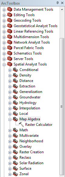
- Click on "Customize" -> "Extension"; and then click on the "Spatial Analyst" to turn on the toolbox.
- Find out the Raster Calculator from Spatial Analyt Tools\Map Algerba\ of the ArcToolbox. This is the interface that allows calculation
of many different operations.
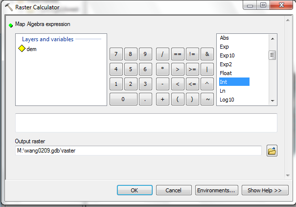
- Click Int and then double-click dem. The expression means
"take the dem raster grid, create a new raster grid called based
on the cell values, but convert the floating-point values to integer values
on a cell-by-cell basis." This is a local function, meaning each cell
value is calculated independently.
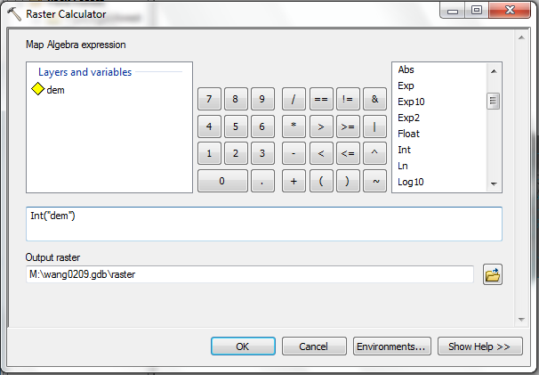
- Click OK. After a few moments the calculation will complete
and the new grid will be added to the data frame.
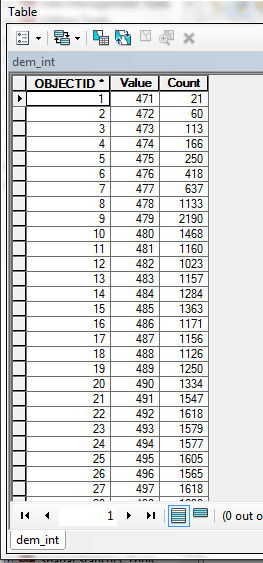
- The grid VAT is different from the vector tables you have seen before.
Rather than a one-to-one feature-to-record relationship, a VAT is simply a
frequency table, showing the number of cells with a given value. For example,
there are 21 cells with elevation value 471 ft.
You have just converted from floating-point to integer value. Be aware that
this conversion may incur a loss of information. Be very careful when converting
floating-point to integer value, especially if your original values are between
0 and 1. You will lose most of your information content. If your data represent
values for which decimal places contain important information (e.g., pH) and
you convert to integer values, you will lose that important information.
A common technique to handle this problem is to first multiply the floating
point raster grid by a 1 or more orders of magnitude, which brings all values
above 1, and then convert to integer value. However, you will need to remember
that the values you now have are not the original values.
Query a raster grid layer (integer data type only)
- Attempt to run a query against the dem_int grid (Selection
> Select By Attributes). You will see that there is no choice for the
grid layer. Close the dialog.
- Instead, from the Table, select Options > Select By Attributes.
This will allow you to create a query on the raster.
- Create a query to select cells in the range from 1000 to 1500.
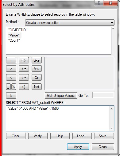
- You can see on the map where these cells are located, and the table also
shows an active selection of 499 records. This is the set of cells with elevation between 1000 and 1500.
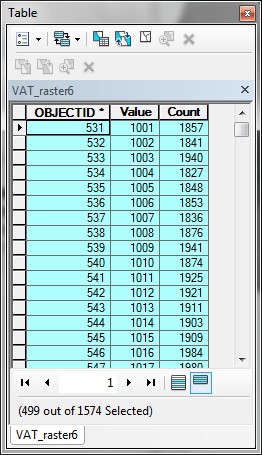
- How much area is in this selection? Perform a Statistics on the Count
field (MGH lab computer will not be able to see the graph here, but the graph will be able to show in any other computer.):

There are 1648088 cells in the selection, which, considering a cell is 100 ft^2, translates
to about 5.9 mi^2 (calculate this on your own now so it will be easier when
you are asked to do this on an assignment!).
- Clear the selection on the table before proceeding.
This query is possible only because the raster grid layer dem_int
raster dataset has a attribute table. This means you cannot perform queries
on floating-point grids.
View a histogram for cell value distribution
Histograms graphically display the spread of cell value data within the selected
cells of a raster grid layer. Histograms can be viewed in layer Properties.
- Open the Properties for Calculation (Symbology > Classify).(MGH lab computer will not be able to perform this process, please read through it.)
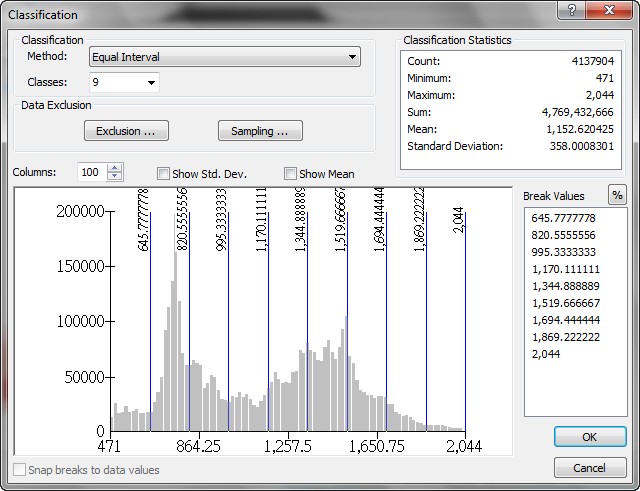
- The elevation values are displayed on the X-axis, and the number of cells
is displayed on the Y-axis. You can see there is a bimodal distribution, with
one peak around 700 ft and another near 1400 ft.
Histograms are useful for browsing the range and distribution of data in a
raster grid. Do the values of a raster grid follow a normal distribution, or
is there some other type of pattern? What might that tell you about your data,
and what implications does it have for further analysis?
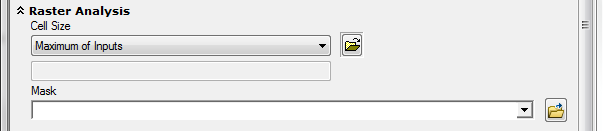
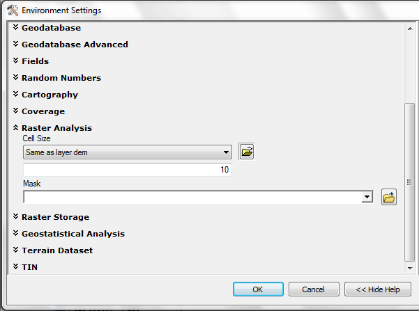
Set analysis properties
Setting analysis environment for raster analysis (Workspace, Processing Extent, Output Coordinates, and Raster Analysis with Cell Size and Mask setting) will affect the analysis
environment until the analysis properties are changed again.
Workspace
The workspace specifies the default location for outputs.
Raster Analysis-Masking
Masking sets the output raster grid to the valid cells of another raster grid.
For every grid, there are cells containing value (e.g., elevation). But there
are also no data cells. Masking allows the output data to be restricted
only to cells containing value in the mask grid. The idea is similar to masking
an area for painting.
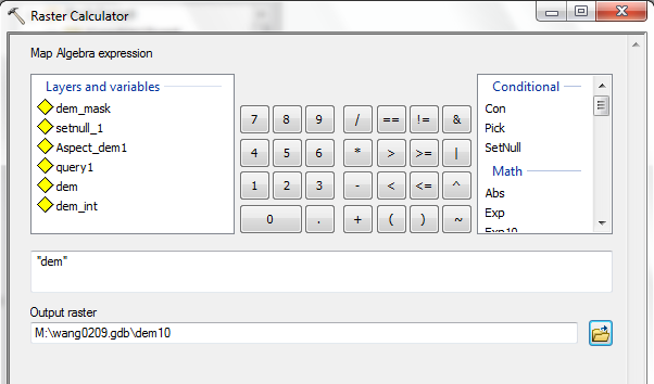
- First, we need to create a raster grid for masking. Generate 500-1000ft raster layer by using Raster Calculator
- Open ArcToolbox and Select Spatial Analyst Tools > Map Algebra > Raster Calculator.
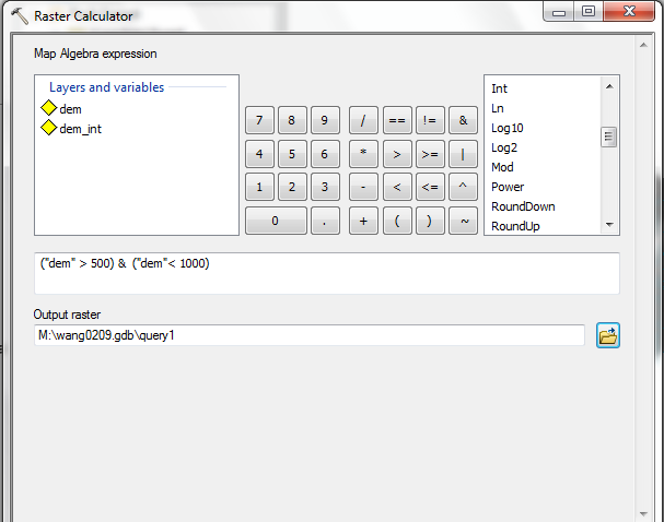
- In the Raster Calculator, using the bottons to click the formula -- ("dem" > 500) & ("dem" < 1000)
- Save this file as Query1 in your M:\ drive and click OK.
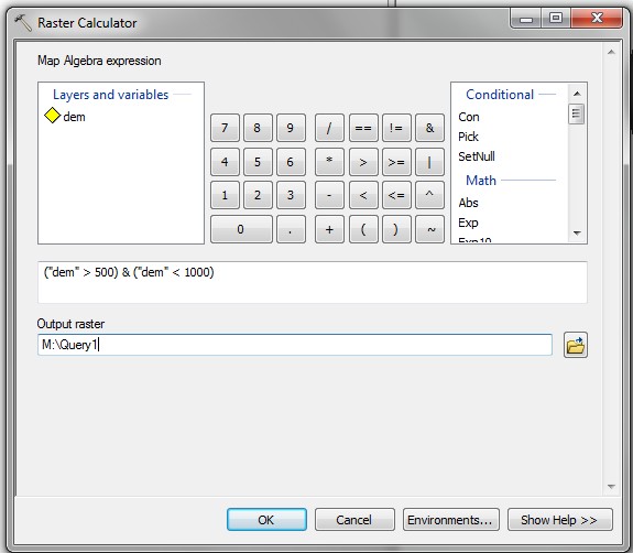
- This step will create
a grid containing only those cells in the 500-1000 ft elevation range.
- Open ArcToolbox and select Spatial Analyst Tools > Conditional
> Set Null.
- The Input conditional raster is Query1.
- The Input false raster or constant value is Query1.
- The Output raster is M:\NETID.gdb\setnull_1.
- The Expression is Value = 0.
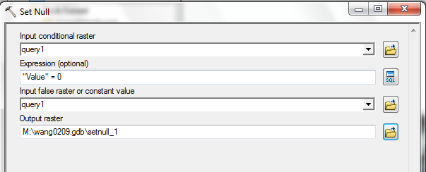
This will create a grid that is identical to Query1, but with NoData values where the original values were 0.
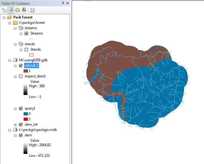
- To see which cells have data and which do not, alter the Properties
> Symbology for the setnull1 layer.
- Select a black shade for the Display NoData as symbol at the
lower right of the dialog.
It is now clear which cells have value and which do not.
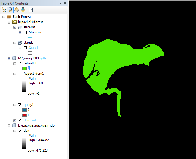
Setting the mask to this grid will mean new grids created using the Spatial Analyst toolbar will have data values only
where setnull1 cells have a value of 1.
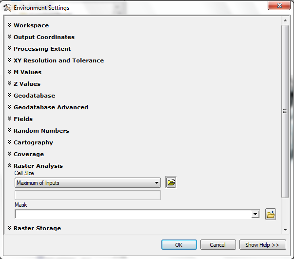
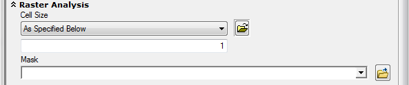
- Select Raster Analysis from Environments.
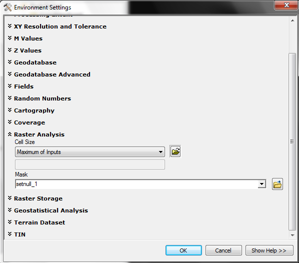
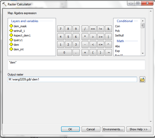
- Perform another Raster Calculation, where the expression is simply [dem].
Using this type of function creates a carbon copy of the original raster grid,
but if analysis properties are set, the resultant dataset will conform to
those properties (cell size, extent, and masking).
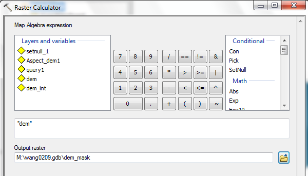
Note that the new raster grid is identical to the original dem grid, but it
contains cells only for those valid cells in the mask raster grid. You should
be able to verify this by looking at the legend (remember, the mask was for
cells in the 500-1000 ft elevation range)..
Processing extent
The Processing Extent is a rectangular area. When the Process Extent is set,
newly created raster grids (from Map Calculations or Map Queries) will be limited
to the spatial extent of that rectangle. The extent can be set to the extent
of an existing layer, to the data frame, to the current display, or to specific
coordinates. The extent is different from a mask, as the mask is defined by
valid cells from a specific grid, whereas the extent is simply a set of rectangular
coordinates.
- Zoom into an area in the middle of the forest (roughly outlined below).
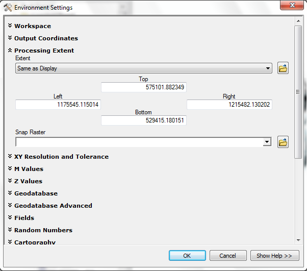
- Alter Processing Extent from Environment Setting.
- Click the Processing Extent tab and select Extent: Same As Display,
which will limit the output of subsequent operations to the current zoom
extent.
- Select Snap Raster: dem. This will make it so that the output
grid lines up with the cells of the dem grid. When you do this, your Analysis extent may change to As Specified Below. This is OK. Still make sure you originally selected Same As Display.
- Click OK.
- Perform another simple calculation as before:
- You will see that a new grid has been created. This grid is limited by the
effect of the mask and the extent. As you can see, only part of the
grid has data.
- Click the Fixed Zoom Out button to verify that the analysis extent
has indeed limited the output to a rectangular area.
- Change the mask setting back to None.
- Perform the same calculation as before ([dem]). Now you can see that
the analysis is still limited by the extent, but not by the mask. Thus, masking
and extent are separate limitations that can work independently or simultaneously.
Analysis Cell size
There is always a tradeoff between data storage and precision. Smaller cells
means potentially better precision, but also larger files and slower processing.
To see the effect of different cell size on precision, storage, and processing,
perform the same analysis but with different cell size.
- Open the ArcToolbox tool Spatial Analyst Tools \ Map Algebra \ Raster Calculator.
- Click Environments (this is where we will change cell size and extent).
- Change the Processing Extent to be the same as
one of the extent-limited grids from a previous calculation. Also, change Raster Analysis> Cell Size to As Specified
Below and set the value as 10 (that is, cells of 10 ft x 10 ft).
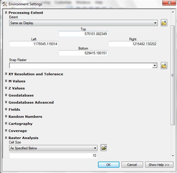
- Put the output in M:\NETID.gdb\dem10.
- Click OK. Write down the amount of time the analysis took (on my
slow computer this was 3 s.).
- Perform the same operation as before, but this time when altering the Environments. Set the Extent as before. but reset the cell size as to 1:
- Put the output in M:\NETID.gdb\dem1.
- Make a note of how long this analysis took. Also, look at the file sizes of these two layers from properties . There
is over an order of magnitude size difference between these data sets.
(My observation: dem1-6.8GB, dem10-28.13MB)
- Going up to a larger cell size should take less time, and the resultant
data sets should be smaller.
There is no hard and fast rule for deciding on a proper cell size. Basically,
you will want to use the largest cell size you can that still correctly represents
the phenomenon you are modeling.
Raster Calculator (I): Perform a map query on a raster grid layer
Many raster grid analytical operations are performed by using the Raster
Calculator tools. Raster grid analysis will be covered in greater depth
in the next lecture, but this section serves as an introduction to these tools.
Because the dem grid layer is stored floating-point, a normal tabular
query is not possible; instead, a Map Query must be performed to view
a subset of cells.
- Open the Raster Calculator (ArcToolbox> Spatial Analysis Tools > Map Algerba > Raster Calculator) and create an expression using the buttons
or keyboard:
("dem" > 500) & ("dem" < 1000)
Your calculation should look like this:
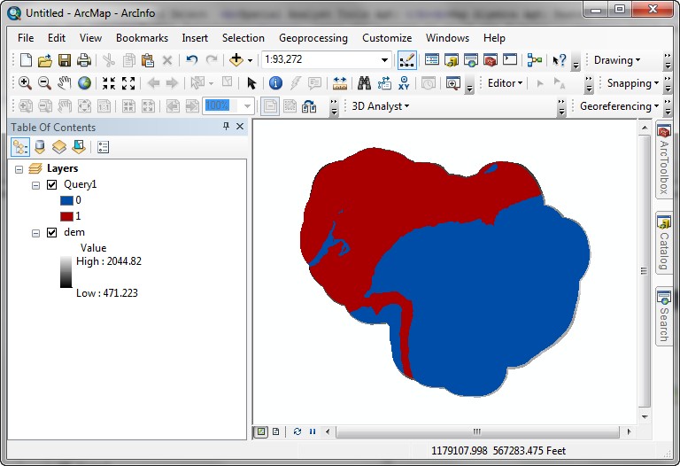
This is a true/false expression. Either cells will be in the 500-1000 range
or they will be outside this range.
- Click OK. The new layer will look like this:
Those cells that matched the expression are given a value of 1, and those
that are either lower than 500 or higher than 1000 are given a value of 0.
A map query is similar to a normal feature layer query, but can be performed
on either floating-point or integer raster grid layers. A map query is similar
to a feature layer query, but the output is always a new raster grid, rather
than a selected set within an existing table. The output is a Boolean entity,
in which output cells are coded True (1) (meeting the query criteria),
False (0) (not meeting the query criteria), or No Data.
Map queries, unlike feature queries, are not limited to single layers. Because
individual cell values are referenced to their spatial position only, map queries
can select cells that match a broad range of criteria, including multiple raster
grid layers. The query above could just as easily have asked to identify cells
matching multiple criteria for any of the raster grid layers within the view.
For example, it is possible to select a group of cells whose values are within
a range of bathymetry in an bathymetry raster grid and whose values
are within a range of slope in a slope raster grid, and whose values
are within a range of salinity values in a salinity raster grid with an expression
like
([depth] < 20) & ([slope] > 5) & ([salinity] < 0.015)
In a typical tabular query, the query is performed on a single table. In the
case presented above, it a query that simultaneously finds cells that match
the value of several raster grids (not just values in a single table). The cell
locations are determined by the spatial referencing framework, but the
values are determined by different values across multiple raster grids.
Raster Calculator (II): Perform a map calculation on a raster grid layer
This example will find the sine of the aspect for each cell in the dem
raster grid. Generating sine and cosine of aspect would be the first step to
take if you needed to perform particular analyses modeling surface terrain,
such as determining insolation, which depends on the angle of the sun. We won't
do anything further with this example, but you should be aware that trigonometric
and other mathematical functions exist for raster grid map calculations.
- Generate the Aspect Layer: Select Spatial Analyst Tools\Surface\Aspect. Select
dem as the Input Surface.
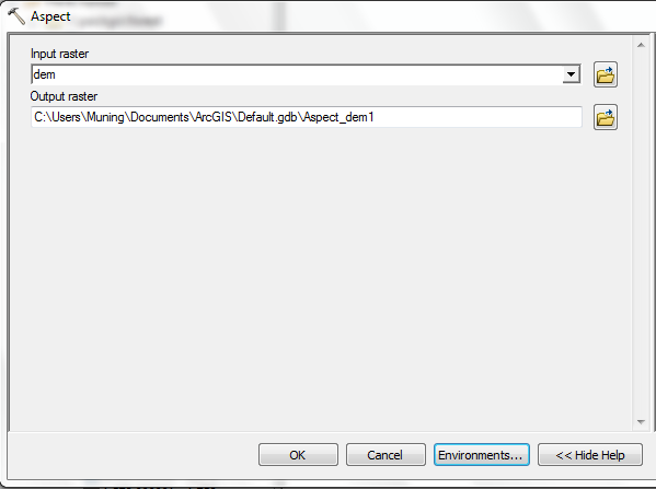
- Click on the Environments..., then set up 1)Workspace as "M:\", and 2) the Cell Size of the Raster Analysis section. In the cell size, select the "same as layer dem"
- This creates a new raster grid, Aspect of Dem1. Aspect is the
compass direction of the steepest downward descent from a cell center. Imagine
dropping a bowling ball and taking the compass bearing of its downward path.
Aspect is a focal function, where the direction of descent for each cell is
determined by the differential elevation of neighboring cells. You will notice
that the Aspect calculation takes longer than the simple local functions we
performed previously.
- Create a new Raster Calculator expression.
- Put the "Aspect of Dem1" raster dataset in the Calculator.
- Select the Sin function from Trigonometry
category .
- Type or build (or copy and paste from the web browser to the calculation
entry control) the following calculation:
Sin("Aspect of dem1" * 3.14159 / 180)
This creates a new grid where first the aspect is converted from degree measure
to radian measure (aspect * pi / 180) and then the sine is calculated, on
a cell-by-cell basis.
Note: Although building calculations and queries is made easier
with the GUI, you can alternatively simply type in the calculation without
using the GUI, assuming you know how to use the proper syntax. Be especially
careful of the location of parentheses.
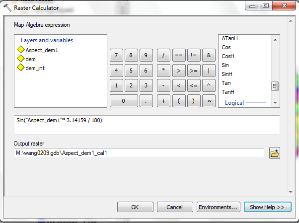
The output is stored in a new temporary raster grid called Aspect_dem1_cal1. The values range from -1 to 1, which is what we should expect for values
of sine.
The Raster Calculator is used to create new datasets based on logarithmic,
arithmetic, Boolean, exponential, relational, and trigonometric functions. These
functions can be performed on individual raster grids or combinations of raster
grids. In addition to the listed operators and functions on the Raster Calculator
interface, any ArcGrid raster grid class functions can be performed using the
dialog. The output of is a raster grid where each cell value is the result of
mathematical or other raster grid functions performed on the input(s).
Advanced use of the Raster Calculator requires learning a little about the
syntax of grid map algebra.
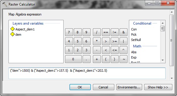
Raster Calculator (III): Querying across multiple grid layers
Perform a complex query that identifies cells that meet multiple criteria across
several grid layers. In this example, find all areas that are
above 1500 ft in elevation and aspect layer (Aspect of Dem1) is South (value 157.5-202.5).
- Add the grid layer Dem from the data CD to a New Dataframe.
- Add the grid layer Aspect of Dem1 from previous exercise.
- Perform a Raster Calculator with the following syntax:
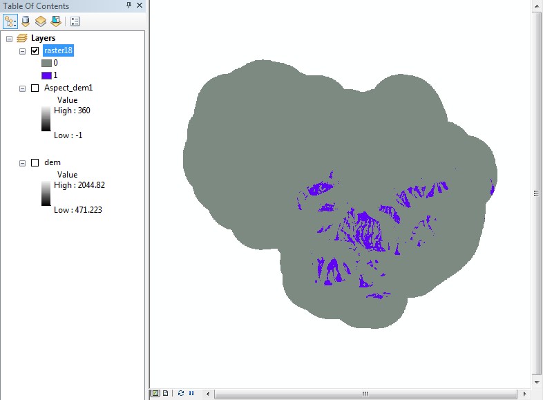
- The output grid shows those cells that matched the logical criteria (value
= 1) and those that did not (value = 0).
- What is the total area of this zone?
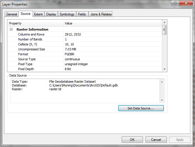
- Open the Properties for the new layer, and make a note of the
cell size (in this case, the cell size is 10).
- Open the attribute table for the new layer (please drag "Count" column wider to see the whole value)
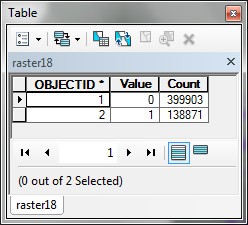 ---->
----> 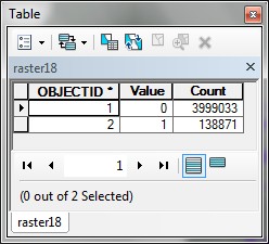
There are 138871 cells (value 1, fit in the query) which are above 1500 ft
in elevation and the aspect is South.
138871 cells * 10 ft * 10 ft * 1 ac / 43560 ft^2 = 318.8 ac.
You have just performed a "query" that picks out cells that match
criteria from more than one grid. This is very similar to the topological overlay
analysis of intersection. Do you see how much more rapid this type of analysis
is with raster analysis? How many separate single actions would it have taken
to do this with vector data? Using more complex syntax within the Raster Calculator
would have allowed us to perform the analysis with even fewer steps.
Although the vector data analyses take advantage of the better representation
of shape for line and polygon features, if the cell size is small enough to
correctly represent the shape of features, the numbers generated will be within
an acceptable margin of error.
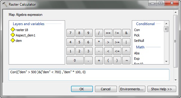
Raster Calculator (IV): Conditional processing
Suppose you have a vegetation model that includes an elevational response factor.
If elevations are between 500 and 700 feet, the model inputs will be 100 * the
elevation value. If the elevations are outside this range, the model inputs
will be 0.
- Add the grid layer Dem from the data CD to a New Dataframe.
- Enter the following expression (feel free to cut-and-paste, remembering
to use the standard <CTRL-C>, <CTRL-V> cut and paste
keystrokes).
con (("Dem"> 500) &
("Dem" < 700),
"DEM" * 100,
0)
The expression means this line-by-line, in English:
If elevation is greater than 500 and less than 700, then
set output value to (elevation * 100), or else
set output value to 0
The output grid will look something like this (adjust the color ramp from the properties to show the difference).
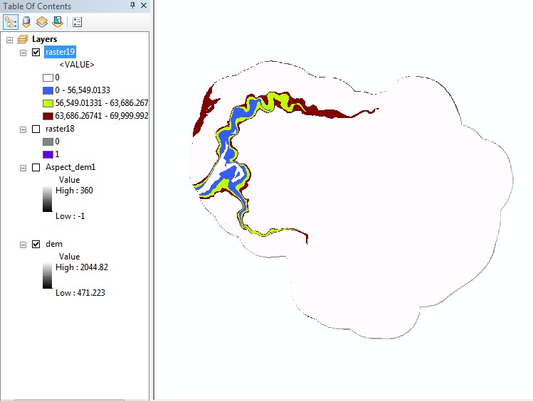
Note that the low and high elevations have an output value of 0, with the
values of the original 500-700 now in the range of 5000-7000. Use the Identify
tool to investigate individual values.
You have just used conditional processing to create a new grid. The actual
values we used are meaningless, but the theory is important. Do you see how
this is different from either a simple reclassification or a map query? A reclass
with this precision would have taken quite some time to code, and a map query
would have given us only yes-or-no values.
The syntax of the conditional statement takes a little getting used to, but
you can see what a powerful tool this is for dealing with conditional processing
of cell values. Frequently in modeling spatial phenomena, we want to treat a
subset of cells in one way and a different subset of cells in a different way.
Please delete any stray files you may have created on the hard drive.
REMEMBER TO TAKE YOUR CD AND REMOVABLE DRIVE
WITH YOU!!!!
Return to top
 |
|
The University of Washington Spatial Technology, GIS, and Remote Sensing
Page is supported by the School
of Forest Resources
|
|
School of Forest Resources
|
 UW
Home
UW
Home