Introduction to Geographic Information Systems in Forest Resources
| Introduction to Geographic Information Systems in Forest Resources |
|
|||||||||||||||
|
|||||||||||||||
Raster analysis is similar in many ways to vector analysis. However, there are some key differences. The major differences between raster and vector modeling are dependent on the nature of the data models themselves. In both raster and vector analysis, all operations are possible because datasets are stored in a common coordinate framework. Every coordinate in the planar section falls within or in proximity to an existing object, whether that object is a point, line, polygon, or raster cell.
In vector analysis, all operations are possible because features in one layer are located by their position in explicit relation to existing features in other layers. Inherent in the arc-node vector data model is chiralty, or left- and right-handedness of arcs (as shown in the polygon data model image from Spatial Data Model). As a corollary to this, containment and overlap are inherent relationships between layers. For example, a point on one layer is on one side of an arc in another layer, or inside or outside of a polygon in yet another layer. The complexity of the vector data model makes for quite complex and hardware-intensive operations.
Raster analysis, on the other hand, enforces its spatial relationships solely on the location of the cell. Raster operations performed on multiple input raster datasets generally output cell values that are the result of computations on a cell-by-cell basis. The value of the output for one cell is usually independent of the value or location of other input or output cells. In some cases, output cell values are influenced by neighboring cells or groups of cells, such as in focal functions.
Raster data are especially suited to continuous data. Continuous data change smoothly across a landscape or surface. Phenomena such as chemical concentration, slope, elevation, and aspect are dealt with in raster data structures far better than in vector data structures. Because of this, many analyses are better suited or only possible with raster data. This section and the next section will explain the fundamentals of raster data processing, as well as some of the more common analytical tools.
ArcGIS can deal with several formats of raster data. Although ArcGIS can load all supported raster data types as images, and analysis can be performed on any supported raster data set, the output of raster analytical functions are always ArcInfo format grids. Because the native raster dataset in ArcGIS is the ArcInfo format grid, from this point on, the term grid will mean the analytically enabled raster dataset.
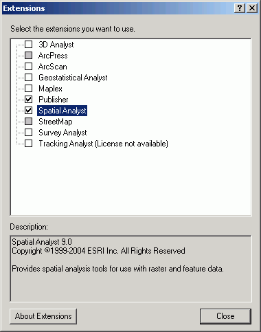
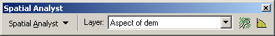
ArcGIS 's interface to raster analysis is through the Spatial Analyst Extension. The Spatial Analyst, when loaded, provides additions to the ArcGIS GUI, including new menus, buttons, and tools. The features added to ArcGIS with the Spatial Analyst are listed here.
OverviewSetting grid layer and analysis properties
Grid layer properties
Adding grid layers to data frames
Displaying grid layers
Examining cell values in grid layers
Managing grid layer files
Grid function typesCell size
Analysis extent
Masking
Local functionsPerforming grid analysis
Global functions
Zonal functions
Focal functions
Map Algebra
The map calculator
Grid layers
Overview
Grid layers are graphical representations of the ArcGIS and ArcInfo implementation of the raster data model. Grid layers are stored with a numeric value for each cell. The numeric cell values are either integer or floating-point. Integer grids have integer values for the cells, whereas floating-point grids have value attributes containing decimal places.
Cell values may be stored in summary tables known as Value Attribute Tables (VATs) within the info subdirectory of the working directory. Because the possible number of unique values in floating-point grids is high, VATs are not built or available for floating-point grids.
VATs do not always exist for integer grids. VATs will exist for integer grids that have:
It is possible to convert floating-point grids to integer grids, and vice versa, but this frequently leads to a loss of information. For example, if your data have very precise measurements representing soil pH, and the values are converted from decimal to integer, zones which were formerly distinct from each other may become indistinguishable.
Grid zones are groups of either contiguous or noncontiguous cells having the same value.
Grid regions are groups of contiguous cells having the same value. Therefore, a grid zone can be composed of 1 or more grid regions.
Although Raster Calculations (which will be discussed shortly) can be performed on both integer and floating-point grids, normal tabular selections are only possible on integer grids that have VATs. This is because a tabular selection is dependent on the existence of a attribute table. Those grids without VATs have no attribute tables, and are therefore unavailable for tabular selections.
Grid layer properties
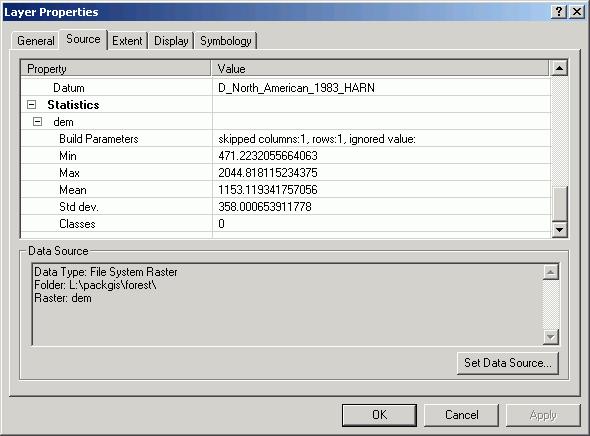
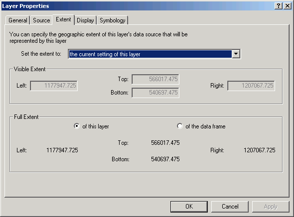
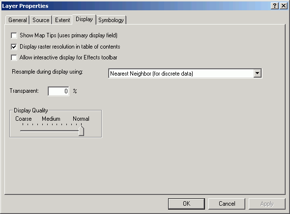
Grid layer properties can be determined by viewing Properties.
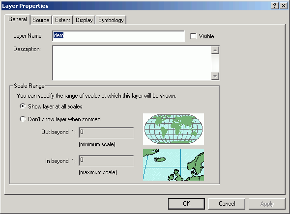
The General tab shows the Layer Name as it appears in the Table of Contents
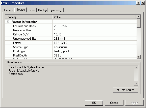
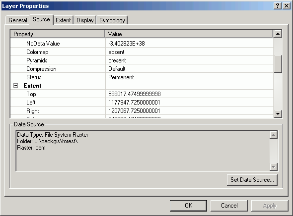
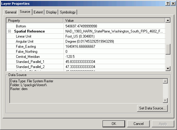
The Source tab shows the Data Source file location and a number of other pieces of information, such as the Cell Size, the number of Rows and Columns, the grid Type (Float or Integer), and the Status (Temporary or Permanent).
The Extent tab shows the lower-left and upper-right coordinates.
The Display and Symbology tabs are used to alter the display of the layer.
Adding grid layers to data frames
Grid layers are added to data frames in the same manner as feature or image
layers, by using the File > Add Data menu control, the Add Layer
button ![]() ,
or by dragging from ArcCatalog. Grid data sources can be added to any ArcMap
document. However, in order to load grid data sources for analysis into a data
frame within the map document, the Spatial Analyst Extension must be
loaded.
,
or by dragging from ArcCatalog. Grid data sources can be added to any ArcMap
document. However, in order to load grid data sources for analysis into a data
frame within the map document, the Spatial Analyst Extension must be
loaded.
Also, in order to access many Spatial Analyst functions, it is necessary to add the Spatial Analyst toolbar.
If the Spatial Analyst Extension is not loaded, it is still possible to add grid data sources to a data frame, but only as simple images. Image layers cannot be queried or analyzed in any way. Image layers are usually not associated with any meaningful attribute values, other than a simple numeric value used for color mapping.
Displaying grid layers
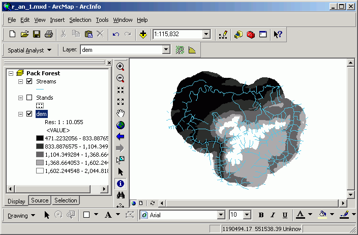
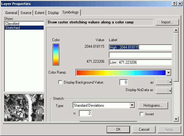
Grid layer displays are altered in almost exactly the same manner as feature layers. Changes to the display of grid layers are done using the Legend Editor. Like polygon feature layers, shading of fills can be changed by altering the symbols of individual classes, by changing the Color Ramp, legend labels, and classification properties. One exception is that grids cannot be displayed with anything other than a solid fill symbol.
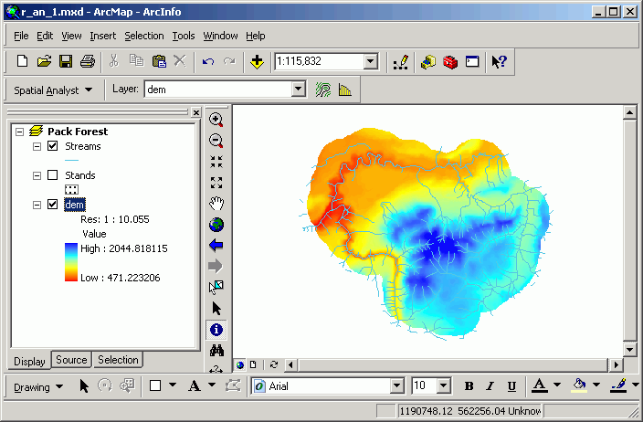
Here, the Pack Forest elevation floating-point elevation grid is displayed with in 5 equal-interval, natural breaks classes, with a gray monochromatic color scheme. Note that the No Data class is not included in the 5 classes.
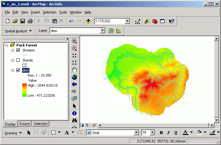
Here the legend has been changed to a Stretched Color Ramp (an option not available for vector data).
Examining cell values in grid layer
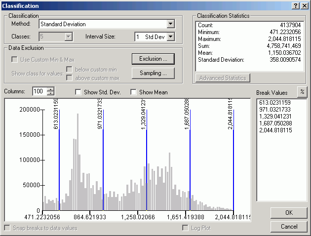
As with vector data, to see the spread of values for a grid, view the layer properties. The histogram displays cell values on the X-axis and cell counts on the Y-axis.
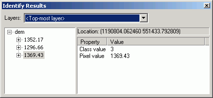
For all grid layers, individual cell values can be queried using the Identify
tool ![]() .
Clicking on a cell for the active grid layer will display the attribute values
for the layer. The Identify Results dialog will display the name of the
grid layer, the X and Y coordinates of the cell, and the cell's value.
.
Clicking on a cell for the active grid layer will display the attribute values
for the layer. The Identify Results dialog will display the name of the
grid layer, the X and Y coordinates of the cell, and the cell's value.
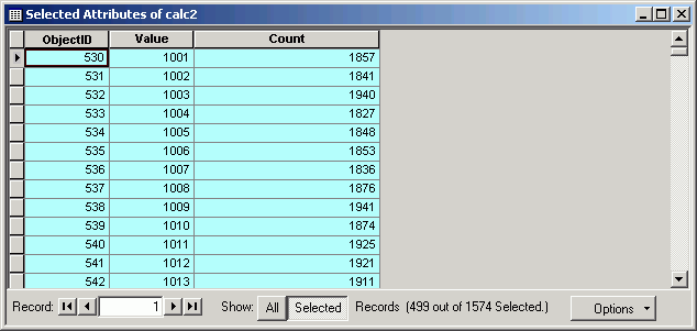
For integer layers with VATs, it is possible to perform tabular selections. Here are all cells with an elevation between 1000 and 1500 ft. In order to make the selection it is necessary to open the VAT and perform the Select By Attributes in table Options.
As with normal feature layer selections, cells meeting the query criteria are displayed in the default selection color.
Managing grid layer files
When the Spatial Analyst performs operations that create new grids on the fly, these new grids are by default temporarily stored in the working directory. If the layer is deleted from the data frame, the grid will also be deleted from the disk. Frequently, grid queries and analyses are not formatted properly in order to obtain the desired result. The incorrect grid can be deleted from the map document, and it will also be removed from the file system (unlike shapefiles, which need to be manually deleted). After the correct result is obtained, the new temporary grid can be saved permanently. In order to make sure that newly created grids are saved, right-click and select Make Permanent. When you do save grid layers, you can choose the file system directory and the name of the layer, rather than accepting the default name and location of the dataset assigned by ArcGIS.
If there are permanently stored grids in a map document, and these are deleted from the map document, they will not be automatically deleted from the disk. If you want to delete the data source you will need to manually delete in the same manner that you manually delete shapefiles or other data sources (that is, with ArcCatalog). Be aware of this, because grid dataset files are very large in size, and can easily fill up a drive, especially a puny 128 MB removable drive.
In order to be able to copy, rename, or delete a layer, all references to the layer must be removed from the map document. Sometimes, even if the layer is removed from the data frame and the attribute table is deleted, ArcGIS "holds on" to a layer. In these cases, it becomes necessary to completely close a ArcGIS entirely before a data source can be deleted.
If you need to delete a grid data source, never use the operating system, use only ArcCatalog. Otherwise you will end up corrupting the file system by leaving "junk" data in the info directory. Cleaning up after this requires the use of ArcInfo's command-line interface.
There are limitations for storing grid data sources you should be aware of:
No spaces in directory or file names! This is a requirement of the complete pathname to a grid data source. Here is an unacceptable pathname:
C:\projects\data\grid data\soil_loss
and an acceptable pathname
C:\projects\data\grid_data\soil_loss
13 character limitation on grid names. Here is an unacceptable grid name:
universal_soil_loss_grid
and an acceptable name:
usle_grid
Names cannot start with a numeral. Here is an unacceptable grid name:
10_meter_dem
and an acceptable name:
dem_10_meter
Setting grid layer and analysis properties
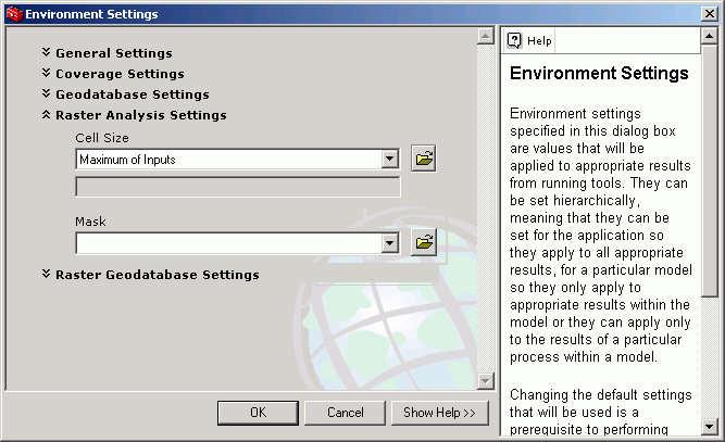
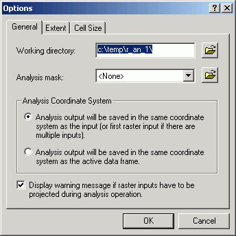
When new grids are created by spatial analysis operations, the user can choose some of the output properties of the created grid. The properties are set by selecting Tools > Options > Geoprocessing > Environments from the menu. After the analysis properties are set, and the map document is saved, the same properties will be used for every analysis within the map document until analysis properties are changed.
Other analysis options can be set using the Spatial Analyst toolbar's Options. The various Analysis Properties can be copied from existing layers, or entered manually.
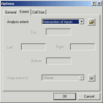
Analysis extent
The spatial extent of the analysis determines the rectangular coordinates of the spatial limit of the output grid will be. It is possible to set the analysis extent manually to any valid coordinates, to the data frame's or display's extent, or to the spatial extent of a layer within the data frame, or to a data source on disk.
Output data will be generated only for the cells within the Analysis Extent. This is frequently used when you are interested in analyzing a small area, rather than performing the operation over the entire study area. The Analysis Extent is a simple rectangle. If you wish to limit the output to match a specific shape of an existing grid, use a Mask.
You should also beware that altering the analysis extent may also alter the registration of grids. If you create a new grid from an existing grid, but with a different analysis extent (even if the cell size is the same), the two grids will not overlay properly unless the analysis extent has an origin that is located at a cell corner for the original grid. This can have significant effects on further processing, calculations, and measurements.
Although acting on a smaller analysis extent can speed things up quite a bit, you should keep a single analysis extent for all processing if you can afford the time and disk space. It is always possible to clip your data down after processing, but if you want to expand the spatial limits of data that are already truncated, you will need to perform the analyses over again.
The red rectangle indicates an analysis extent:
An analysis is performed, and then the display is zoomed to the extent of the output:
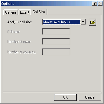
Cell size
Existing grids are stored with a certain known cell size. You can check the
cell size of any grid layer in Analysis Properties. It is preferable when performing
multi-grid analyses to choose an output cell size that is the same as the largest
of the input cell sizes. It is always possible to decrease information
content by resampling cells to a larger cell size, but it is impossible to increase
information content by splitting cells. Because the individual cell is the smallest
resolvable feature in a grid, although the software will allow it, it is ill-advised
to subdivide the cell into different values.
Remember that cell size is the measurement of the edge of a single cell, not
the area of a cell. Also remember that cell size is stored in the map units
for the dataset. For the Pack Forest data, that unit is always feet.
So a grid that has cells with a size of 10 means cells measure 10 x 10, or 100
square units.
Number of rows and columns
The number of rows and columns can be automatically determined by the combination of cell size and bounding coordinates. Or the number of rows and columns can be set manually, in which case the cell size will change to accommodate the new number of rows and columns.
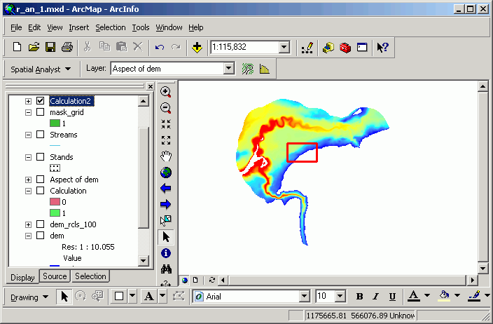
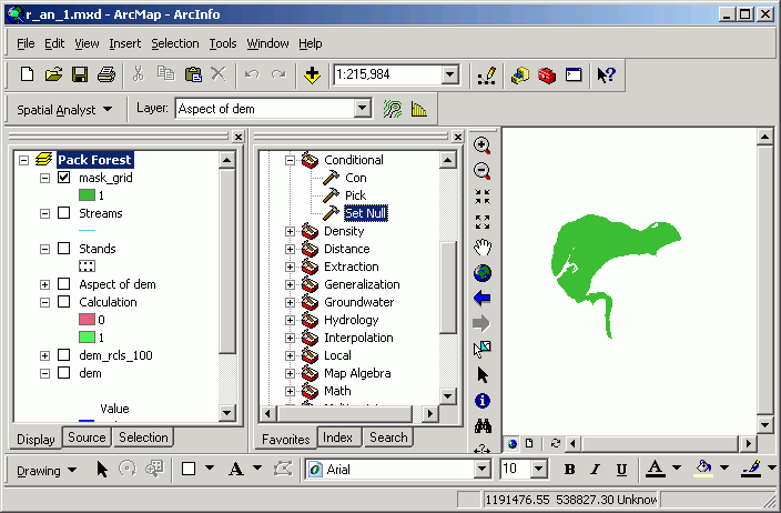
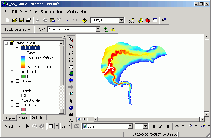
Mask grids can be used to limit the spatial output to the non-null extent of an existing grid layer. Calculations will occur for the cell locations that have valid values in the mask grid. In the following example, a mask grid has been prepared representing a certain area of the forest:
Performing an analysis, the output is limited only to the unmasked area.
There are three basic categories of functions for the creation of new grids: global, focal, and zonal.
Local functions
Most grid operations perform their algorithm on every cell in the dataset. You can think of the local function calculation engine as starting at once cell location, performing a calculation once on the inputs at that location, and then moving on to the next cell location, and so on.
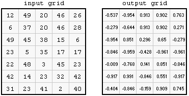
Here is a global function, where the individual output grid cell values are the result of the local sine function performed on every input cell:
Most of the functions that create new grids based on analyses performed on vector layers are local functions.
Global functions
Global functions perform operations based on the input of the entire grid. Functions such as calculating distance grids and flow accumulation require processing of the entire grid for creating output.
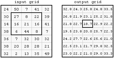
Certain grid operations do consider neighborhoods, so that the output cell is the result of a calculation performed on either a group of cells determined by a window of cells (known as a kernel or focus) around the cell of interest. These operations are called focal functions. For example, a smoothing (low-pass filter) algorithm will take the mean value of a 3-x-3 cell kernel, and place the output value in the location of the central cell. If the kernel contains locations that are outside of the grid, these locations are not used in the calculation.
In this focal mean example, the outlined cells in the input grid are averaged, and the resultant value is placed in the center cell of the kernel in the output grid. This is done for every 3-x-3 neighborhood in the input.
Zonal functions
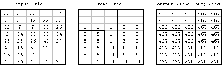
Other operations perform functions based on a group of cells with a common value (a zone) in one of the inputs. The group of cells are known as zonal functions, since they calculate single output values for a group of cells based the location of the input zone.
Here, the zones are defined by the zone grid. The function is a zonal sum, which sums all the input cells per zone, and places the output in each corresponding zone cell in the output. The zone boundaries are included only for illustrative purposes, and are not actually part of the dataset.
Raster analytical functions are performed in a number of different ways:
We will cover various types of raster analysis in the next section.
Spatial Referencing
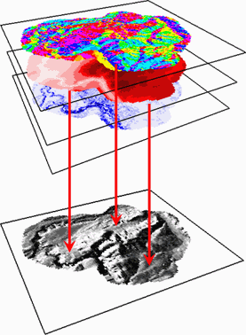
Raster analyses that use multiple grids are possible because of the spatial referencing of grids to a common coordinate space. This is similar to how multi-layer analyses are possible with vector data.
In the image above, a process uses 3 input grids and creates a single output grid. The analysis is performed on a cell-by-cell locational basis, where the calculation is performed on each value from the 3 input grids. Output from the calculation is placed at the same location in the output grid.
Map Algebra
For most grid functions, other than those which simply identify a selected group of cells, operations take the conceptual format of an algebraic expression. For this reason, the syntax of grid analytical operations is often referred to as "map algebra." Sometimes map algebra uses functional notation:
output_data_set = function (input_data_set(s) {,arguments})
For example, to generate a slope grid from an elevation grid, with values in percent:
slp_grid = slope (dem, percentrise)
Sometimes map algebra takes the form of arithmetic expressions:
output_data_set = input_grid1 operator input_grid2 ...
For example, to calculate the multiplication of the two input grids slp_grid and dem:
slp_dem = slp_grid * dem
Usually the input and output datasets are grids, but they can also be vector datasets, such as polygonal zones or isoline layers.
Map algebra statements and other analytical functions are created using special tools, such as the Raster Calculator and Map Query, in the Spatial Analyst-enabled GUI.
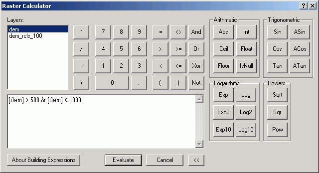
The Raster Calculator
The Raster Calculator is the main interface for performing Map Algebra.
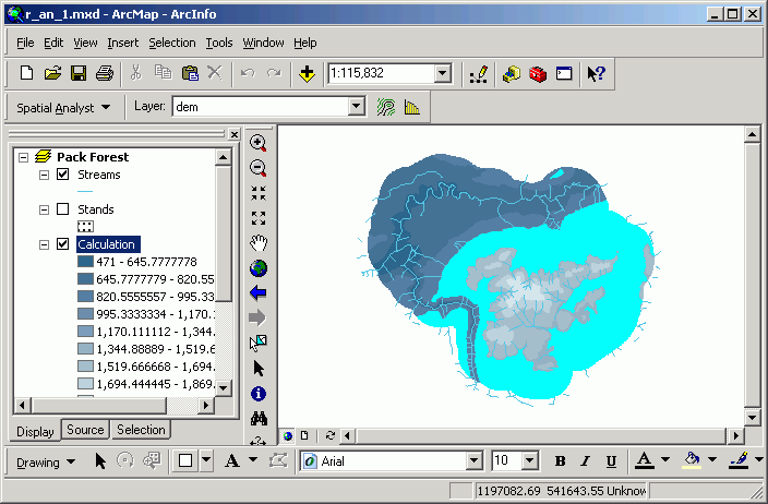
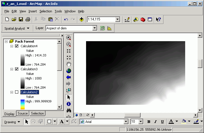
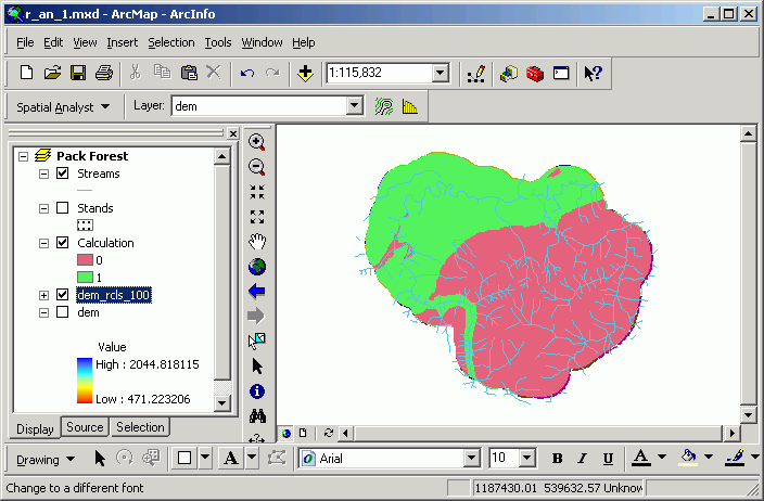
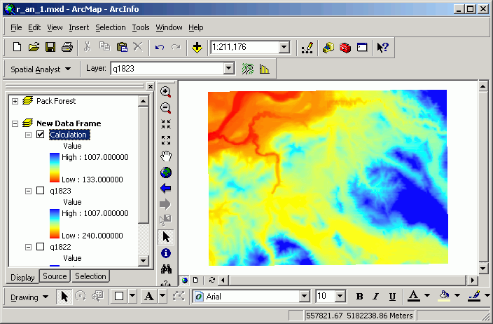
Here are images from 2 data frames that display the input and output of this analysis:
Note in the second image, the Calculation grid has values that display the results of the Boolean operation (1 = yes, 0 = no).
The Raster Calculator contains controls for selecting Layers (which can be thought of as values in the Map Algebra expression), Numbers, and Operators. There are different classes of operators (Arithmetic, Relational, Boolean, Logarithmic, Trigonometric, Powers). The expression area is where you build the Map Algebra expression, either by clicking on parts of the GUI, or by writing a valid ArcInfo Grid map algebra expression.
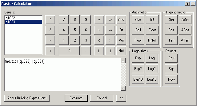
In our next lab session we will also be using the Raster Calculator to perform a Map Algebra function for mosaicing:
Translated to Map Algebra:
Map Calculation 1 = mosaic (eaton, elbe)
Which essentially creates a new grid called Map Calculation 1 that is the result of performing the mosaic function on the elbe and eaton grids.
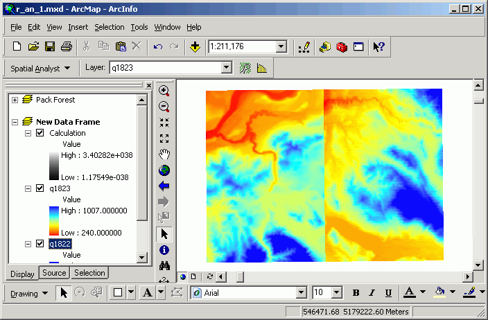
Here is the result of this analysis:
In the first image, 2 separate grids exist. After the Mosaic operation, Calculation includes all cells from the 2 inputs.
We will cover additional raster operations in the next lesson as well.
Return to top | Ahead to Help Topics
|
|||||||||||||||
|
The University of Washington Spatial Technology, GIS, and Remote Sensing Page is supported by the School of Forest Resources |
School of Forest Resources |