
Introduction to Geographic Information
Systems in Forest Resources |
Creating and Modifying
Tables
Objectives:
- to become familiar with tabular operations in ArcGIS
- to create graphs from tables
- Perform drive
substitution to create drives L (CD) and M (removable drive).
- Clear out the M: drive
- Adding and Editing Tables
Copy a file to your personal directory
Start ArcGIS and open an existing map document
Add a table to the map document
Change the attribute title in the table
Edit and add any single record
Add fields and calculate values
- Selecting and Summarizing Records
Query a table and display the selected set
Get descriptive statistics on the selected set
Modify a selection
Summarize a table
- Joining and Linking Tables
Join tables
Use a joined field for layer display
Link tables
Remove links and joins
- Create a Graph
Create a graph for selected features
Graph multiple fields
Change the graph type
- Export a graph
- Export a table
- Close the map document
Perform drive substitution
Perform drive
substitution to create the virtual drives L and M.
Clear out the M: drive
- Delete or Move everything from the M: drive and your geodatabase so you will have enough space to work
through this exercise. (Suggetion: Create a geodatabase in your own computer and move the files)
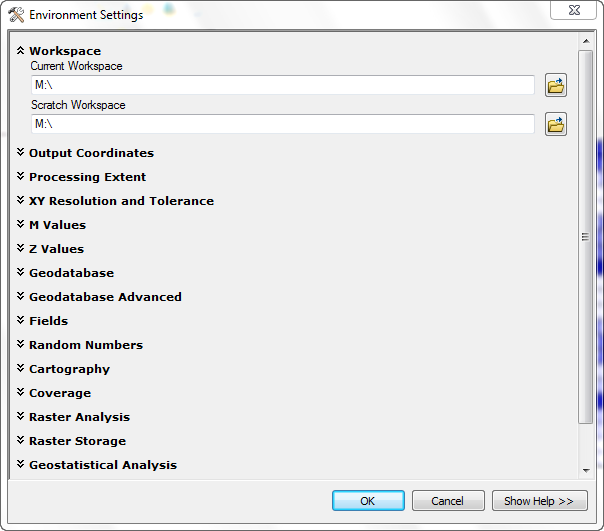
- Also take this opportunity to set your current workspace to the M: drive
(Geoprocessing > Environments > Workspace
).
Adding and Editing Tables
Copy a file to your personal directory
- Download the file plots.zip and save it on the M: drive. This is a self-extracting
zip file of a dBASE table containing reference trees for the Pack Forest Continuous
Forest Inventory plot centers.
- Double-click on the file name in the Windows Explorer to extract the file.
Extract it to the M: drive (not to the default location). After you have extracted
the file you will see a file called plots.dbf.
- Once it is uncompressed, it will open in ArcMap without any translation,
i.e. no need to import or convert.
Start ArcGIS and open an existing map document
- Retrieve the map document tables.mxd and
save it in your personal directory.
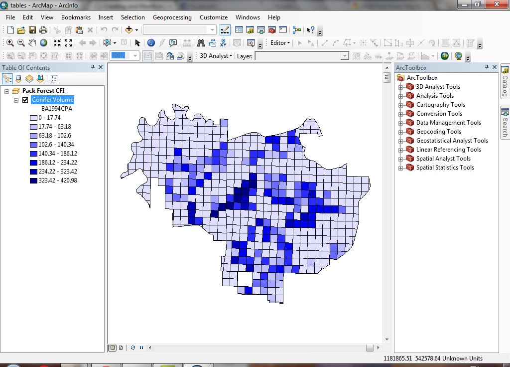
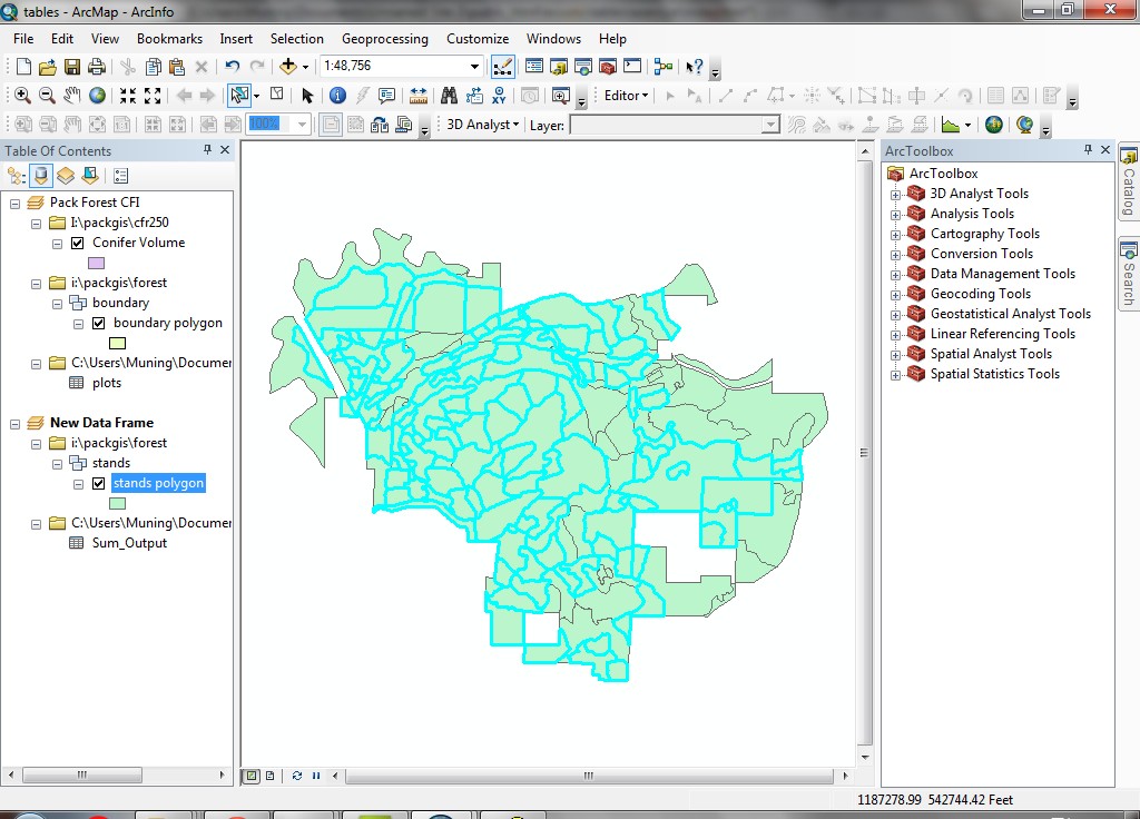
The map document will open with a view document containing the Pack Forest
CFI layer.
Add a table to the map document
- Add the table to the map document by using Add Data...
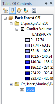
- You will see the table has been added by checking the List by Source button
in the Table of Contents.
- Right-click and Open the table.
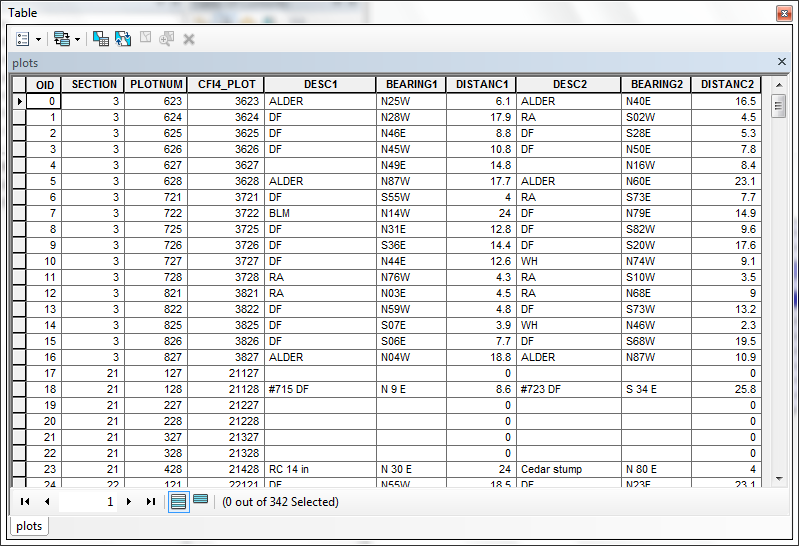
You have just downloaded a table from the web and added it in to an ArcMap
document. Most of the tables we have used up to now are feature layer attribute
tables. However, any supported (text, dBASE, or INFO) files containing tabular
data can be added in the same manner.
Change the attribute title in the table
Tables can be altered within ArcMap, either by editing (as long as it is an
editable data source), which changes the source file (on the disk, ), or by
altering the display properties, such as hiding fields or giving field name
aliases (which does not change the source data).
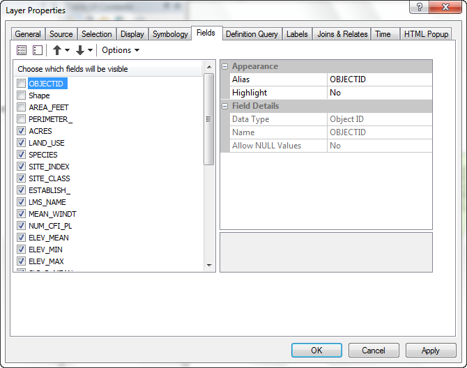
- Change the table's appearance by right-clicking the table in the Table of
Contents and selecting Properties from the popup menu.
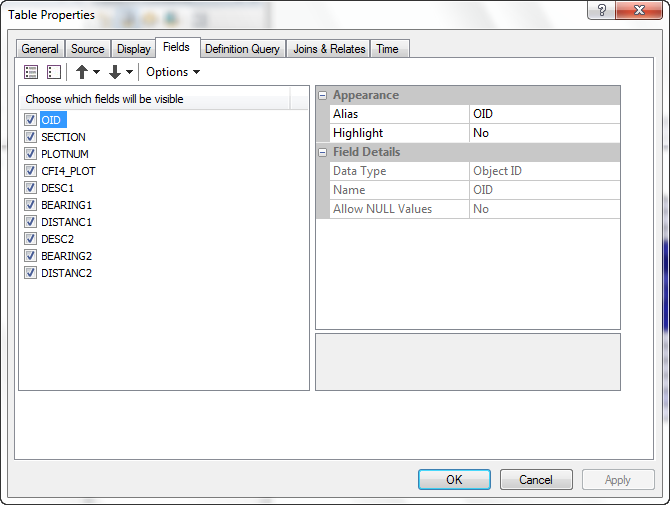
- Uncheck the fields OID, Section and Plotnum, and type
"Plot ID Number" in the Alias field for the Cfi4_plot
field name. Note also that you can see the properties for each field (the
data type, length, precision, scale, number format).
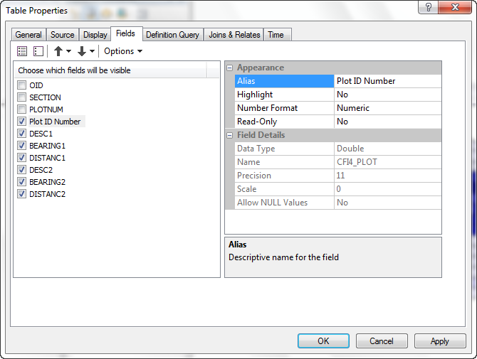
- Click OK to apply these changes.
- This will rename the table, hide the two unchecked fields,
and alter the displayed name of the Cfi4_plot field.
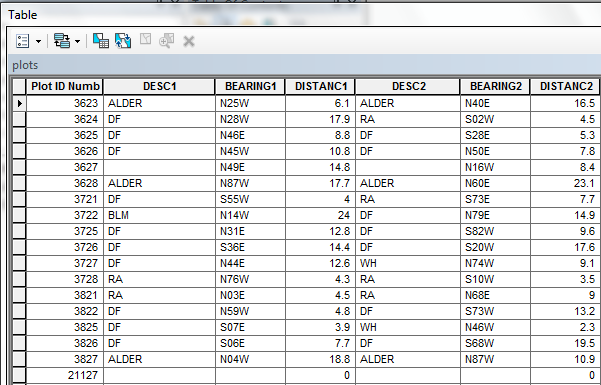
Note that the field name has changed and the unchecked fields no longer display.
You can use this technique to reduce "clutter" and to make field
names more understandable. The field name changes only for this table within
this map document, and does not alter the data source.
You have just altered a table's appearance in ArcGIS by hiding some fields
and creating field aliases for others. Alter the table appearance when you need
to view fewer fields, or if you want to change the names of fields as they appear
in the table document. Remember that changing a table's appearance does not
alter the table's source data.
Edit and add any single record
- Click the Editor toolbar buttom
 is next to scale bar from
the menu.
is next to scale bar from
the menu.

- Select Editor > Start Editing from the menu. Select the polt layer that you will edit.
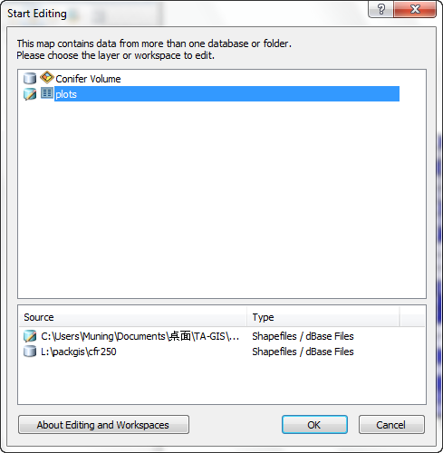
Be aware that you will only be able to edit data to which you
have write-permission. This means that you cannot change tables that are stored
on the CD (you might want to remember this for an assignment)!
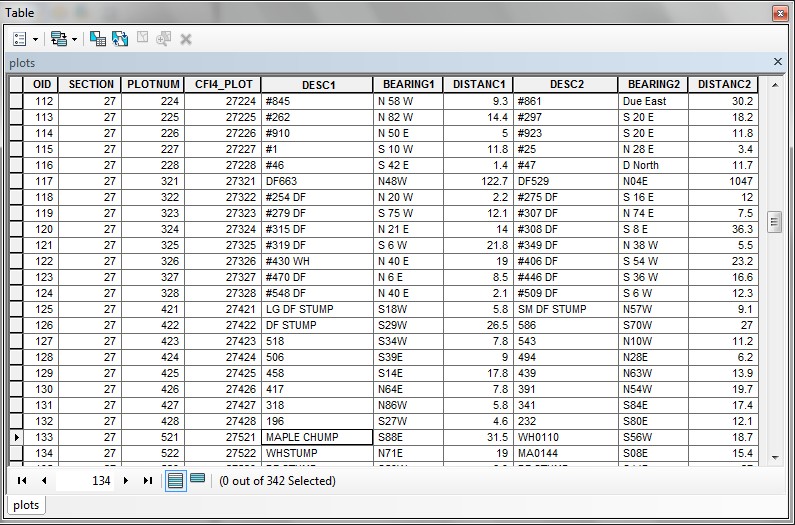
- There are a few records in the table with typographical errors. Find the
record where CLUMP" is misspelled "CHUMP."
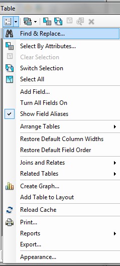
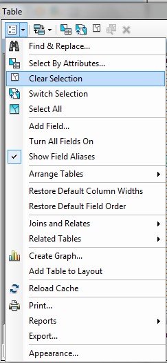
- Use Options
 > Find and Replace.
- Enter chump as the string to find. Uncheck Match Case, then
click Find Next.
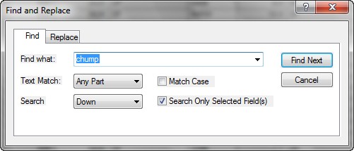
- The cell containing "MAPLE CHUMP" will be shown.
- Change the H to an L and press the <ENTER> key
to apply the change.
-
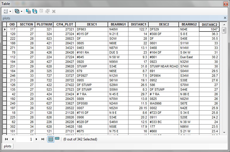
Next, find the record in which the value for
DISTANC2 is too high.
Right-click the field name and then sort it, descending. The record whose
value is
1047 should be fixed to read
147.
- There is one record which was mistakenly not entered. It should have these
values:
| Section |
Plotnum |
Plot ID Number |
Desc1 |
Bearing1 |
DISTANC1 |
Desc2 |
Bearing2 |
DISTANC2 |
| 3 |
828 |
3828 |
DF |
N34E |
13.8 |
DF |
S76E |
28.8 |
- Because the Section and Plotnum fields were hidden previously,
you will need to unhide them (Properties from the Table of Contents,
and check the checkbox for the fields).
- Scroll to the bottom of the table and enter these values.
- Update the values of this record to match the values shown above.
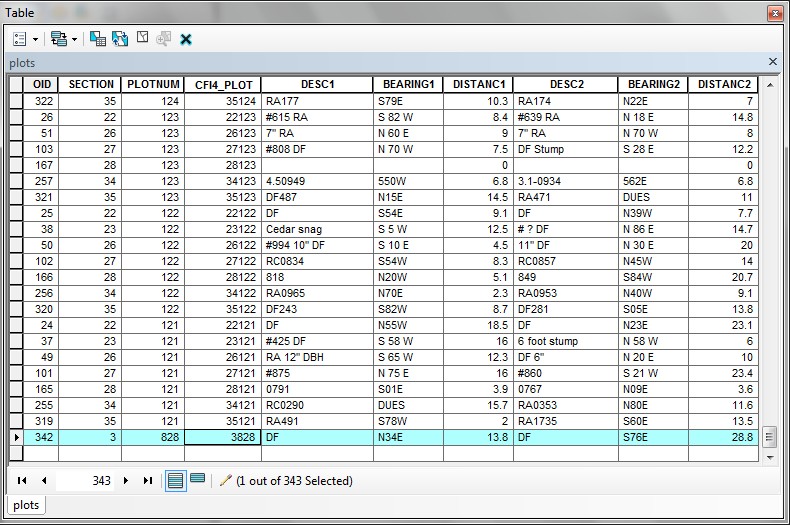
- Click any cell in a different record to set the values.
You have just made single edits to various values in a table. Be aware that
when a table is open for editing, you can alter the value of any cell in the
table, whether a record is selected or not.
Add new fields and calculate values
The current unit of measure for distances in this table is feet. We need to
add fields for the distance in meters for a group of visiting students from
Switzerland. To do this, first add the new fields.
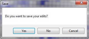
- If the CFI Plot Reference Trees table is open for editing, it must
be set to an non-editable state before adding fields. From the Editor
toolbar, select Stop Editing. When prompted, save the changes.
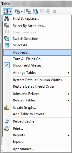
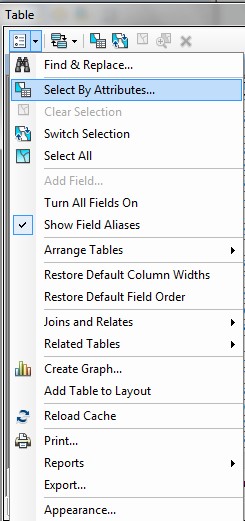
- Click the Options button and Add Field. (Note: Add Field can only be operated when editing tool is closed)
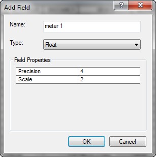
This field will be numeric, with 4 data columns, and 2 decimal places. For
example, you could store these possible values in the field:
Before you add fields, you should consider what data will
be stored in the field. This will determine the field definition. In this
case, I have determined that a locator tree will not be more than 99 meters
from the plot center. Adding two decimal places of precision makes the field
4 columns wide.
- Add the other new field called meters2 with the same field definitions.

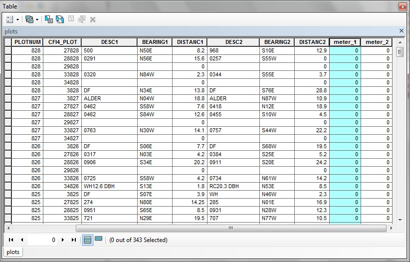
You now have 2 new fields in your table.
Note that when new items are added to the table, values for that field are
null or 0.
- Clear any selected records (if there is any), so the calculation we perform will be applied
to all records in the table.
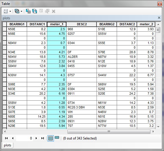
- Drag the field meters1 field title to the left until it is adjacent
to the DISTANC1 field. That way you will be able to see the fields
next to each other.
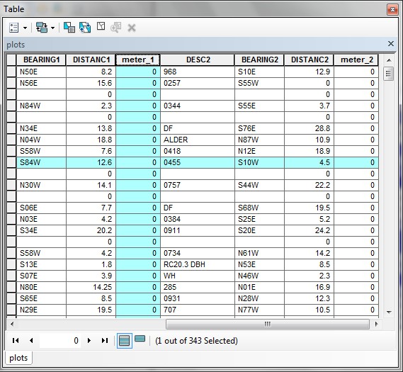
- Right-click the field heading for meters1 and select Field Calculator .
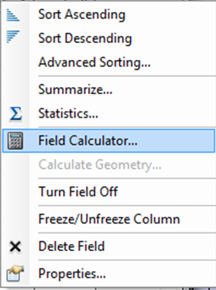
- In the Field Calculator, build the expression by double-clicking
DISTANC1, then entering / 3.2808.
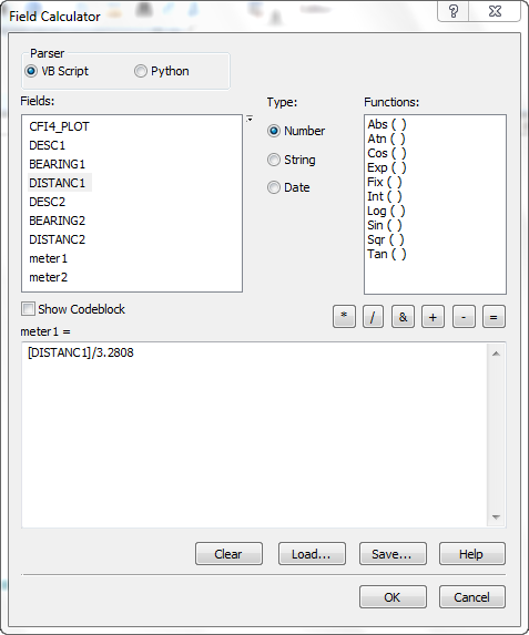
Note it is a mistake to include the meters1 field in the expression.
By making this field active and using the field calculator, you are telling
ArcGIS that you want to calculate values for that particular field. As a reminder,
the Field Calculator dialog shows the name of the field that is being
calculated above the expression text entry control.
- Click OK to perform the calculation.
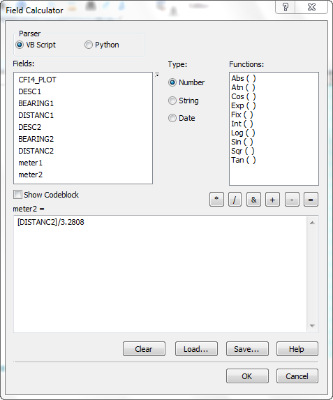
- Do the same for the meters2 field, making sure to calculate using
the DISTANC2 field.
- Scroll around the table in order to see the change. Make sure your values
pass a reality check!
You have just created new fields in the table and used the field calculator
to populate the new fields with values. The field calculator is used when you
want to add values for based on calculations from other fields, or if you want
to add values for several records at a time.
It is possible to perform advanced calculations by using Visual Basic syntax.
To see these options, click Help in the Field Calculator menu.
Selecting and Summarizing Records
Query a table and display the selected set
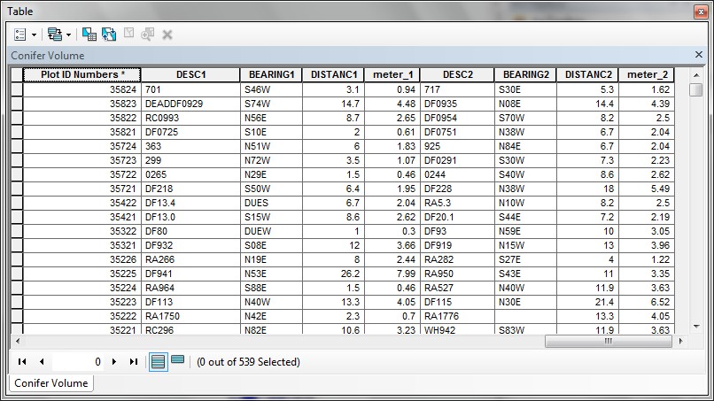
- Open the attribute table for the Conifer Volume (right-click, Open
Attribute Table).
- Scroll through the table to see what items and values exist. The items represent
basal (BA - the cross-sectional area of a tree at 1.2 m) area and Scribner
(board-foot) volume to a 6" top (SV6) for the indicated years.
The items represent either conifer per acre (CPA) or hardwood per acre
(HPA). There are several other items beyond our present concern.
- Select records for plots with high hardwood basal area in 1994 by invoking
the Select by Attributes dialog (Options > Select By Attributes).
[Basal area is a measure of the cross-sectional area of a tree's stem at 1.3
m above the ground.]
- Scroll down to the BA1994HPA (basal area / acre for hardwoods in
1994) item and double-click it.
- Click the > sign, and type in 100. If you make a mistake, highlight
and delete the query and start over.
- The query should look like the image below (with all parentheses and braces
in the right places. Spaces are optional).
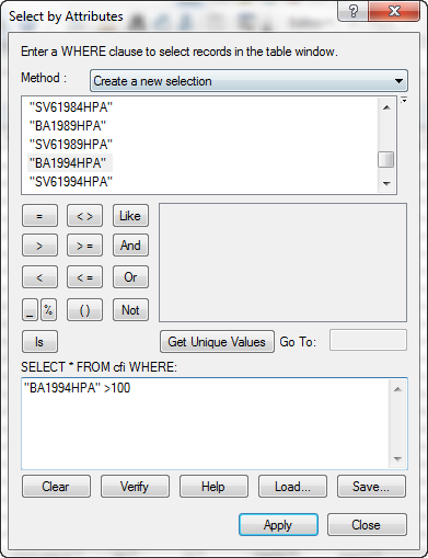
Click Apply and then Close.
It is important to format your query string properly in order to avoid syntax
errors. Also, it is important to select the proper Method. In this
case, we are creating a new selection, so we did not select a different method.
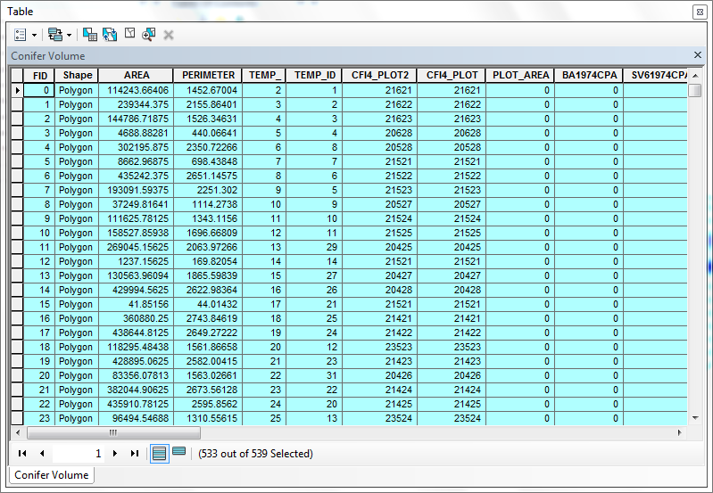
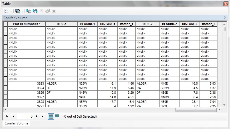
- Several polygons will appear to be selected, but you may not see any records
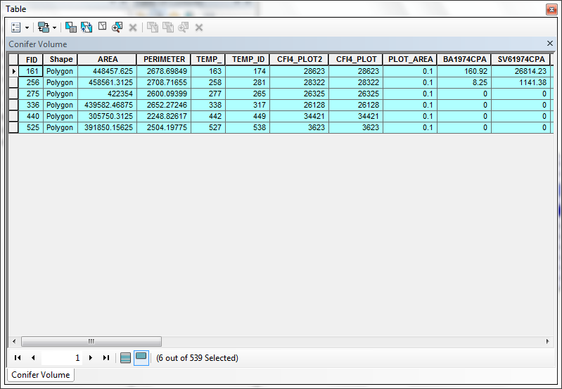
selected (although the table shows that 6 out of 539 records are selected).
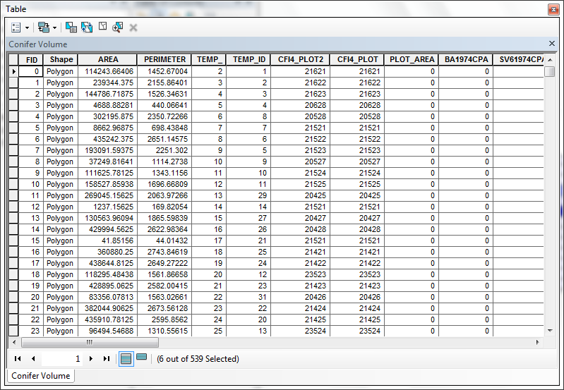
- To see only the selected records, click the Show selected records button. Now
only selected records will be displayed.
- Click the Show all records button to show all records
- Switch selected sets by selecting Options > Switch Selection.
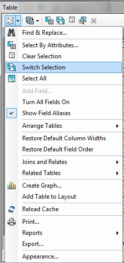
The table will display the opposite selection (533 out of 539 selected).
- Click Switch Selection button again to return to the originally selected
set.
You have just used a logical statement to select out specific records in a
table. In this case, because the table is a feature attribute table,
the corresponding features are selected for the layer in the map display of
the view. You can perform queries on other tables within ArcGIS, regardless
of the source file type.
Get descriptive statistics on the selected set
Now that we can see which records and plots have high hardwood basal area,
we may be interested in other statistics about the data.
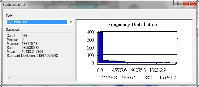
- With the selected set still active, right-click the field representing 1994
Scribner volume for conifers (SV61994CPA) and click Statistics.
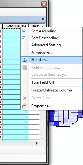
- Descriptive statistics are listed in the popup. Note that these are descriptive
statistics only for the selected set of records/features. (The MGH lab will not display the chart graph due to the technical difficulty)
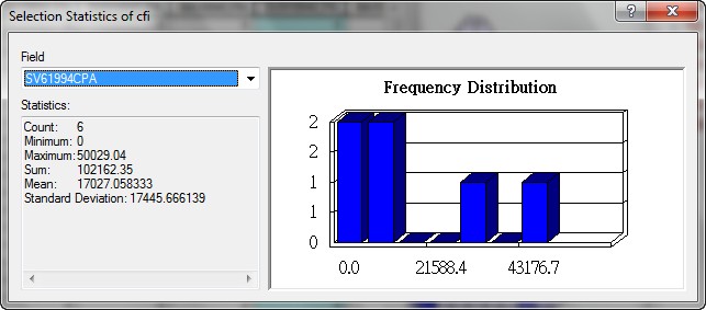
We can see the mean volume per acre for these records is a little more than
17,000 board-feet.
- Close the Statistics dialog.
- Clear the selected set (Options > Clear Selection).
- Generate statistics again. You will be able to learn much about your data
by looking at these statistics (The MGH lab will not display the chart graph due to the technical difficulty).
The mean volume for all plots is about 10,000 bd-ft.
- Close the Statistics dialog.
You have just obtained summary statistics for a numeric field. Understanding
the range and spread of data values for layers is one of the basic things you
should be familiar with. In this, case you calculated summary statistics for
both a selected set of records as well as for all records in the table.
Modify a selection
Sometimes selections are either too broad or too narrow. In the case above,
our selection included plots with no conifer volume at all. We may be interested
in a subset of plots which have high conifer volume and high hardwood
volume.
- First, make a query that selects plots with
hardwood basal area (BA1994HPA) greater than 80, as shown below.
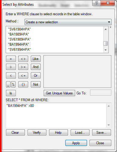
- Click Apply and then dismiss the Select by Attributes dialog.
This selects all plots whose hardwood basal area in 1994 was greater than
80 sq in. This selects 19 polygons.
- We will narrow the selection by selecting out polygons with conifer
basal area (BA1994CPA) greater than 100, as shown below. Formulate
the query in the same manner, but choose the method
instead of the Create a new selection method. If you make a mistake
you can always clear the selected set and start
the query over from scratch.
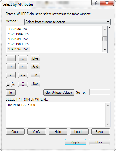
- This selects out only 4 polygons. What kinds of forest management activities
might you suggest for these areas?
You have just performed a 2-step query on a table. You will frequently need
to select records that match a large set of criteria from several fields of
data in the table. Use this technique to pare down your selections. If you need
to add records to or remove records from selected sets, rather than reducing
selected sets, use the Add to or Remove from methods.
Summarizing Tables
Summarizing a table gives you the ability to see patterns in your data which
may not otherwise be evident from looking at a raw table. Summaries work by
acting on the unique occurrences of values within a specified field. Summaries
also allow you to generate summary statistics based on numeric fields within
the table that is to be summarized.
The results of a summary are stored in new tables (i.e., new dBASE files on
the disk), so you need to specify the output directory and filename for the
new table. These tables always contain the summary field, the count of records
for each unique occurrence of the summary field value, and optional summary
statistics.
Summaries also allow you to simplify data in order to create graphs, since
showing too many table values in a single graph can be confusing.
- Insert a new data frame and add the L:\packgis\forest\stands layer
from Add Data button.
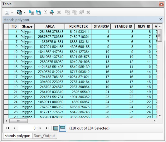
- Open the stands polygon attribute table.
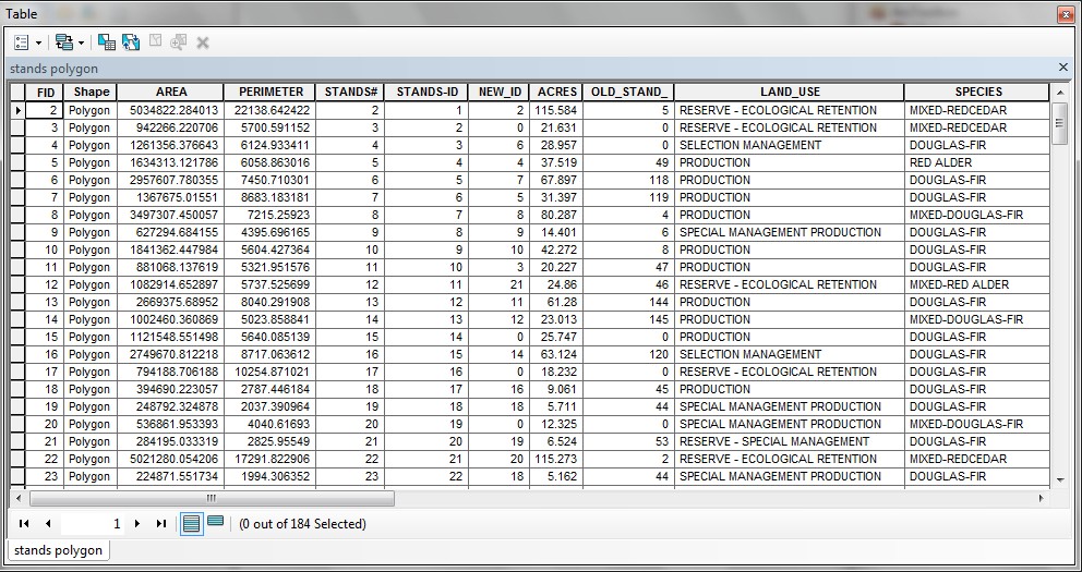
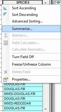
- Make the Species field active, and then right click on the heading of the field Species and choose Summarize
from the menu.
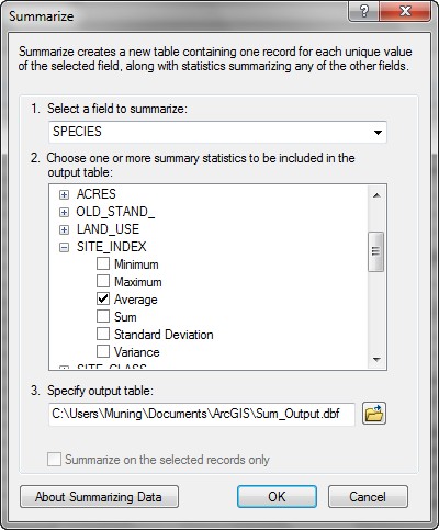
- Add the sum of area to the summary table, as well as the average
site index:
- Check the box for ACRES > Sum.
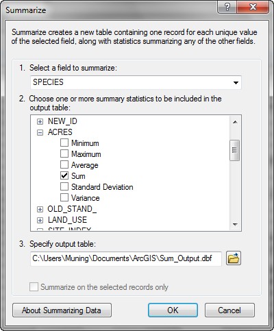
- Check the box for SITE_INDEX > Average. Also specify the output
table as m:\spec_area. ArcGIS will automatically add the .dbf
file extension to the filename when the summary table is created.
You can either type in the path to this new table or use the Browse
button  to navigate to the directory where you want to save the table, and enter
the file name.
to navigate to the directory where you want to save the table, and enter
the file name.
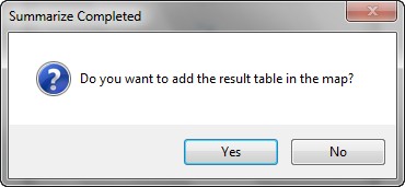
- Click the Yes button to create the table.
- Open the table (note that the table shows up in the Source tab of the Table of
Contents).
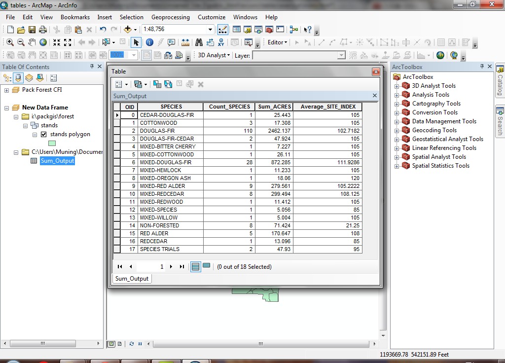
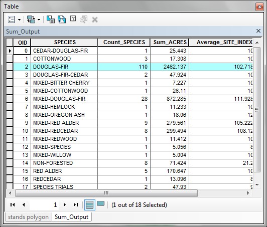
The summary table is automatically added to the map document. It will contain
the fields OID, SPECIES, Count_SPECIES, Sum_ACRES,
and Average_SITE_INDEX. The SPECIES field contains the unique
values of the SPECIES field in the source table. This field exists in
the output table because it was the active field originally; this field is what
we wanted a summary about. Count_SPECIES, which is automatically created,
lists the count of records for each species in the source table. The other items
(Sum_ACRES and Average_SITE_INDEX) represent the sum of acres
and average site index per each species type; these are the individual fields
we intended to generate.
Table summaries also work with selected sets; only selected records will be
summarized if there is an active selection. Otherwise all records in the table
will be summarized.
If you create a summary table without adding any summary statistics, the output
table will contain a copy of the summary field with one record for each unique
value in the summary field as well as the Count field, which contains
values of the number of records for each unique value in the source table.
Joining and Linking Tables
Joins and links are touched upon in the relational
data model. In this example, we have the plot location table as well as
the attribute table for the CFI plots ("Conifer Volume"). The common
field between these tables is Cfi4_plot and CFI Plot ID Number,
which is the plot's identification number.
Joining tables
- Re-activate Pack Forest CFI data frame.
- Right-click the Conifer Volume layer and select Joins and Relates
> Join....
- Select the choices as below. This will join the plots table to the
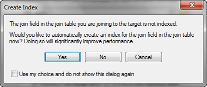
Conifer Volume table, based on the CFI4_PLOT field. Remember that you renamed the CFI4_PLOT field in an earlier step (by changing the alias). This is why you are joining the CFI4_PLOT field to the field Plot ID Numbers (Original CFI4_PLOT in the plots table). Note: Join table needs to have same field from two different table to join. If you joined with two different fields, the joined table will not have any meaning of it.
- Click Yes and create the index when prompted.
- Open the Conifer Volume table. You will see the original fields from the plots table.
- Scroll to the right and you will see the joined fields have been added. For records that do not have a matched value in the joined table,
the values will appear as <Null>. Note: If you place a wrong join, you may see <Null> in almost all records.
The tables have not been physically joined (that is, joined
as a single file on the disk), but are only managed this way by ArcGIS. You
can verify this by adding another copy of the Conifer Volume layer (L:\packgis\cfr250\cfi.shp),
and open its table, which will not contain the additional fields created by
the join.
You have just joined two tables in ArcGIS. Use this technique to increase the
informational content of your layers. You will frequently encounter layer attribute
data that are minimal in content, but can be linked to other tables containing
extended attributes. When a map document is saved, all of the join information
is also saved, so if you open a map document, ArcGIS will reestablish any joins.
Use a joined field for layer display
For most of ArcGIS 's purposes, the resultant table created from a join functions
just like any other table. If the resultant table happens to be a layer attribute
table, then ArcGIS gives you the luxury of displaying or analyzing joined data
as though it were an integral part of your attribute table.
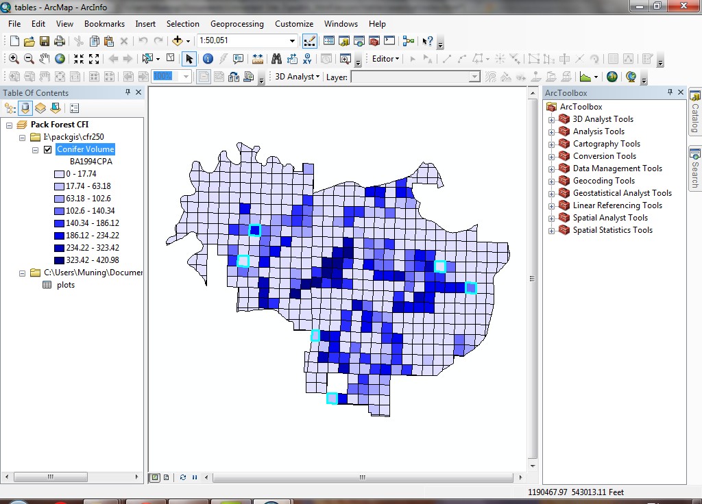
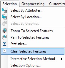
- Make the Pack Forest CFI data frame active, and clear any selected
features (Selection > Clear Selected Features).
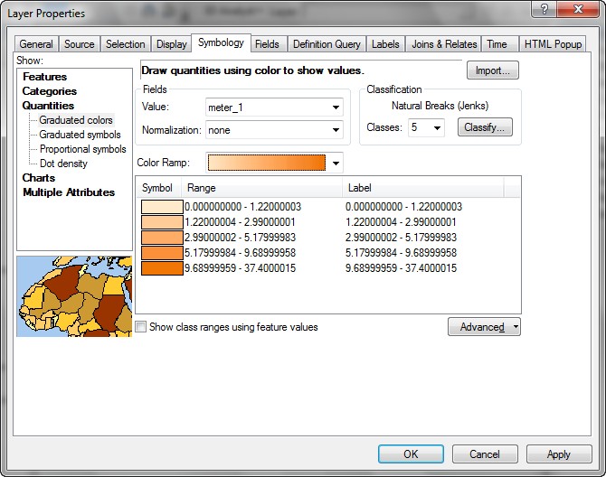
- Change the legend for the layer from layer properties so that it is using a Graduated Color display
with the defaults of Natural Breaks and 5 classes, based on the meters1
field. Select the Color Ramp to orange monochromatic.
- Note that some of the polygons do not appear. These are polygons for which
the classification field is null (there was no match on the join).
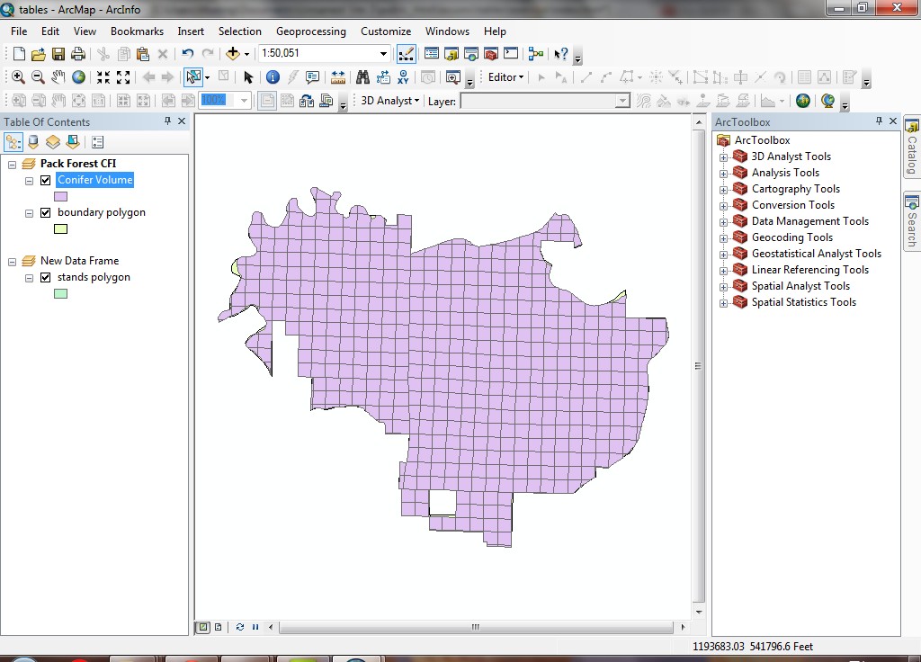
- Add the \packgis\forest\boundary data source as a polygon layer with
a contrasting color and drag the order below the Conifer Volume layer, and make sure it draws before the CFI plots.
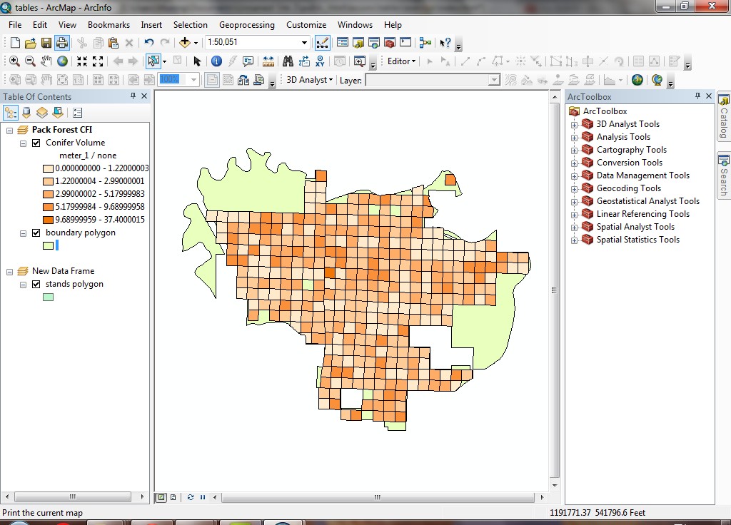
If there is a positive correlation between the distance of plot trees from
the plot center and difficulty in finding the plot center, the darker plots
will be more difficult to find. You might alter your field work schedule accordingly.
Remove relates and joins
If any joins or relates are active, you can easily remove them by making the
tables active that contain relates or joins and selecting Remove Join(s)
or Remove Relate(s).
You will need to do this when your relates or joins have gone in the wrong
direction.
- Remove the join (right-click the Conifer Volume layer name and select
Remove Join(s) > plots.
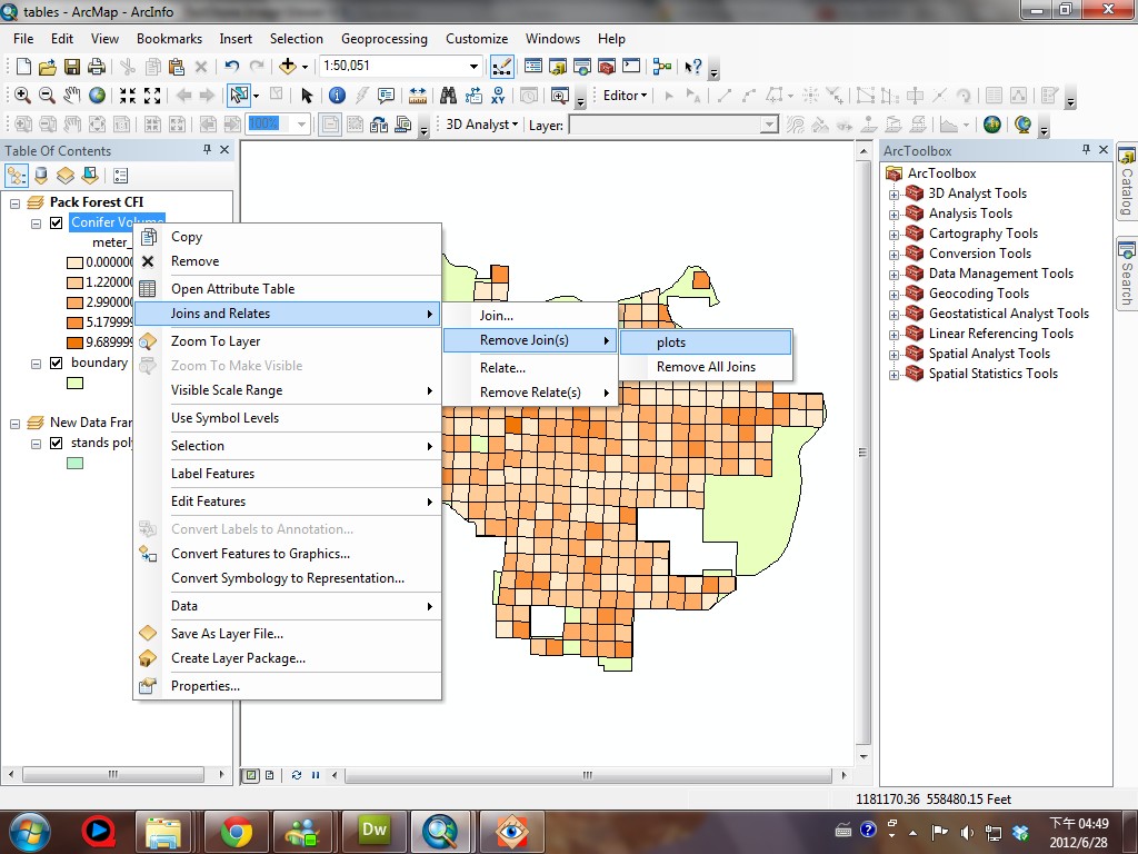
Note that the classification reverts to single symbol because the field previously
used for display no longer exists in the table.
You have just used a joined field for altering a layer's display. If you have
tables of extended attributes that can be joined to your attribute tables, you
can use those extended attributes for display of layers.
Relating tables
Tabular relates are similar to joins, but with relates, the tables remain separate.
However, selected records in one table also select related tables in associated
tables. Also, in contrast to joins, relates are often made between tables which
have a one-to-many relationship. In this section, we will relate a species table
to the stands attribute table. Links are performed when you have a one-to-many
relationship between your destination and source tables.
- Activate the New Data Frame.
- Right-click on the stands polygon layer and select Joins and Relates
> Relate....
- Following the example below, relate the stands polygon table to the table (summarizing from Summarizing Tables exercise) the by the SPECIES field.
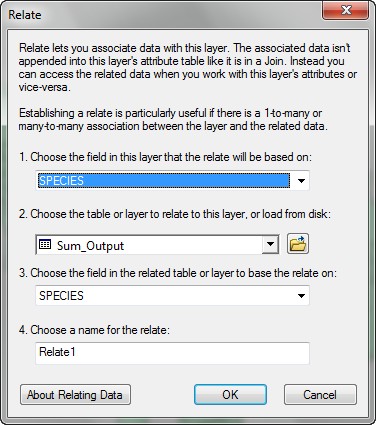
You will not notice any changes.
- From the menu, click Related Tables botton and select Relate1: Sum_Output to open both tables.
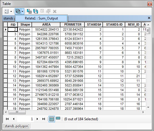
- After that, make a selection from Sum_Output table, select DOUGLAS-FIR from species field.
- Now, click on Related Tables again, you will see all the records with DOUGLAS-FIR species are marked.
Part of the value of relating tables is that it allows you to make very rapid
selections on data. You can easily select, in order, DOUGLAS-FIR stands,
then MIXED-REDCEDAR, then RED ALDER. Imagine how much longer
this would have taken if you had used Select by Attributes to make
a selection based on species.
You have just related tables together. Always use relating when you have a
one-to-many relationship between the destination and source tables.
You can also relate tables together both ways so a selection on either table
will select related records in the other table. Also, you can string relates
together across multiple tables so a record selected on one table will select
records in 2 or more related tables.
Create a Graph
Create a graph for selected features
- Select the records representing REDCEDAR and MIXED-REDCEDAR
in the spec_area table.
Use a query (or use the <CTRL> key to select more
than one record directly in the table).
- From the Options menu, select Related Tables
> stands_species : polygon to select related features in the stands
polygon layer. Your selection should appear the same as the image below.
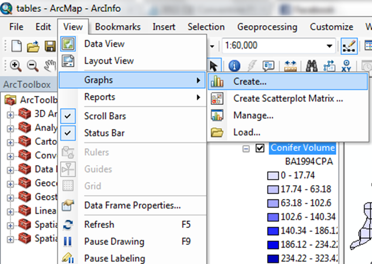
2. Create a graph by selecting View > Graphs > Create.
- Alter the graph parameters:
- Use the default graph type (Vertical Bar)
- Select Value filed: Sum_ACRES
- Select X label field: SPECIES
- Select Color: Palette - Classic
- Click Next.
- Select the radio button for Show only selected features/records on the graph.
- Enter Area by Species as the title.
- For axis properties, enter area (ac) as the axis property title (in the tab for the Left-hand axis).
Your display should match the same image below.
- Click Finish.The graph shows the number of acres in each species
class for the selected set of records.
- Open the table of "spec_area" and go to Options->
Clear Selection
- Right-click on the title bar for the graph and select
Properties....
- Go to Appearance and check "Show all features/records on graph"
and click "OK"
You will need to resize the graph window to see the legend.
You have just created a simple graph from a table. Graphs in ArcGIS are always
derived from tables.
Graph multiple fields
To graph more than one field at a time, alter the graph properties.
- Right-click the title bar of the graph and select Properties. At the bottom of the Series tab. Click the Add button and select "New Series".
-
Note that there are now two series tabs (Vertial Bar and Vertical Bar 2).
- For the Value field in the second series, select Average_SITE_INDEX
- For the Xlabel field, select
SPECIES
- For Color, select Custom and select the blue shade.
- Click OK
- Because the site index values are much lower than the area values, it will
be necessary to alter the data range of the Y-axis. Right-click on the
title bar of the graph window and select Advanced Properties....
- Click Axis on the left-hand pane.
- Click Maximum tab at the middle of the right-hand pane.
- Click Change and enter 500. Click OK and Close
- You will probably need to make the graph full screen in order to see all
the data as well as the species classes. The image below has been reduced to
fit on the web page. This allows you to compare values of different
fields for the same records.
- Open the graph's Properties again, and in the Multiple
bar type section, choose Side All. Click OK.
You have just altered your graph so that it displays more than one field at
a time. Use this method any time you want to compare values among different
fields and classes. Note that the upper bounds of the graph are not shown, which could be misleading (500 is not the maximum extent of the data)!!
Change the graph type
To change graph types, right-click on the top bar and go to Properties.
You have the choice of Area, Bar, Column, Line, Pie, XY Scatter, XY Bubble,
Polar, and Hig-low-close graphs. For graph type, there are
several choices.
- Select graph type and click the Pie graph.
- Click the Data tab and select
Value field: Sum_ACRES
Label field: SPECIES
Color: Palette - Classic.
- Click "OK"
- Right-click the title bar of the graph window and select Advanced Properties.
- Click Pie in the left pane.
Click the Marks tab among the upper tabs in right-hand pane.
Click the Style tab among the lower set of tabs.
- Check Visible and choose Style Label.
- Click Series on the left window. Uncheck Vertical
Bar in the right-hand pane.
- Click Close. Your graph should match the one displayed below.
-
Resize your window to show the labels clearly.
Now your graph shows the proportion of the area taken up by each species
class. You can see that well over 50% of the forest is in the DOUGLAS-FIR
species class. The relative proportions are difficult to determine looking at
the summary table or the column graph, but are readily apparent in the pie graph.
Feel free to experiment with different graph types.
Export a graph
If you want to place an image of your graph in a different application, you
can either export the graph as an image file or copy it to the clipboard and
paste it into another application.
- Right-click the title bar of the graph and select Export....
- To save as a Windows metafile graphic, select Format >
Metafile and click Save....
- Navigate to your M: drive and name the file area_species
- Open Microsoft Word and insert the image (Click Insert > Picture from File).
Navigate to M:\ and you will see the image file.
- Select the image file and click Insert.
Saving the graph as a file will give you a file you can reuse. If you only need to place a graph in another document, and you do not need the graphics file saved, you can use Windows clipboard instead.
- Go back to the graph in ArcMap, right-click the title bar and select Copy
as Graph.
- Switch back to Word.
- Right-click in the document and select Paste to place
the image in the document. The first image is a vector format, while the second
image is a bitmap.
Try zooming in or changing the size of the images in Word
to see how the different image formats differ. Note that the bitmap format
looks "fuzzy" as you increase the zoom factor.
You can export graphs to images for use in other applications. However, once
you do, you will lose the "live link." That is to say, if you go back
to ArcMap and alter the graph, the image file you exported will not change,
so make sure you have made your graph look the way you want before you export.
Export a table
- Perform a selection of all records from the stands attribute table
where the stand age in 2003 is greater than 100.
- Alter the table properties so that several fields are hidden, like so:
- From the Options menu, select Export.
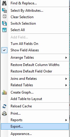
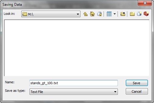
- Click the Browse button, which will allow you to specify the output
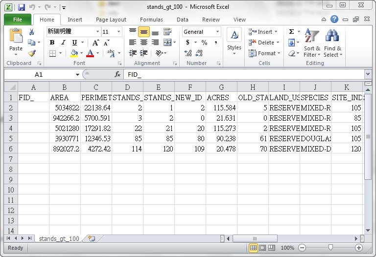
location, file name, and file type.Navigate to M:\, call the file stands_gt_100 and specify
Text File as the export format.
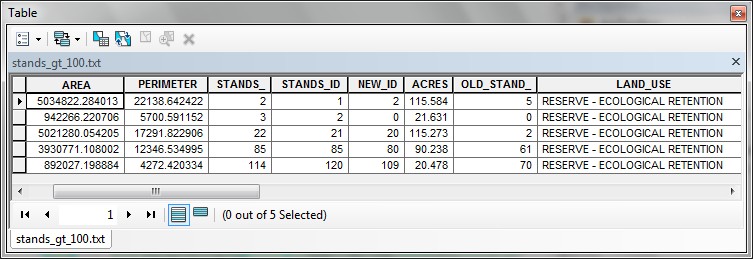
- After the file is created, add it to the map document.
Note you will see the table listed in the TOC in the Source tab. Open the table in ArcMap.
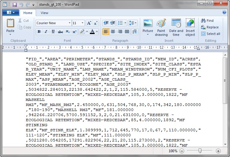
- Open the file from the Windows Explorer. You should see the file open with
Notepad or WordPad. Note that the file only contains the selected records,
and only the visible fields.
- Open the text file in Excel.
You have just exported a table from ArcGIS into a generic format. You can use
this technique to save tables for import into other applications, such as statistical
analysis software.
Close the map document
- Select File > Exit.
- If you wish to save the changes to this map document, choose Yes,
and save the map document on the M: drive. If not, click No.
REMEMBER TO TAKE YOUR CD AND REMOVABLE DRIVE
WITH YOU!!!!
Return to top
 |
|
TThe University of Washington Spatial Technology, GIS, and Remote Sensing
Page is supported by the School of Forest Resources
|
|
School of Forest Resources
|
 UW
Home
UW
Home