Introduction to Geographic Information Systems in Forest Resources

UW Home GIS@UW Search

Syllabus Schedule Class Meetings Assignments Course Data Contact Us CFR 520 Lab Locations Software Collect It Page

One of the most powerful sets of functions in GIS is the ability to manage, display, and analyze surfaces. Raster analysis contains methods for analyzing surface data, as we have seen in previous lectures and exercises. However, although raster analysis contains methods for analyzing and displaying 3-dimensional surfaces, the graphical output is usually limited to planimetric display. A large amount of information is communicated with the use of 3D images.

ArcGIS 's 3D Analyst Extension provides some powerful and impressive tools for analysis and display of 3D surfaces, as well as integration with traditional 2D raster and vector data sources. The 3D Analyst is an extension that adds support for 3D shapes, surface modeling, and real-time perspective viewing to ArcGIS. With it, you can create and visualize spatial data using a third dimension to provide insight, reveal trends, and solve problems.

Here is a typical 3D perspective view of Pack Forest elevation with streams and roads. The view has a 3x vertical exaggeration applied, which makes topographic features more distinct. For skilled map readers, it is easy to visualize the relationship of topography, roads, and streams as a landscape system. However, reading a topographic map requires certain knowledge and experience that not everyone possesses. Even for experienced map readers, an image like this conveys far more intuitive information than a flat paper map.

Frequently, numerical attributes are mapped with graduated color or size symbols to emphasize features with high values. Even these types of maps need some type of intellectual interpretation. ArcScene is usually used to display elevation surfaces, but it can be used to display any kind of data which can be viewed as a response surface. Raster or TIN surfaces establish the 3D framework for the display of raster or vector layers. Vector data raster data sources can be draped over surfaces. Shapes can be extruded up or down, to imply volume height, or depth.

These two images show essentially the same data in the same classification style. However, the use of the third dimension adds more visual impact and communicative power. In the first image population is displayed in a graduated color symbology.

The same symbology is used, but an extrusion proportional to population density is used, effectively showing two variables simultaneously.

Limitations exist for displaying choropleth (graduated color) maps. After about 5 classes are used, the map becomes unreadable, because the reader cannot discern among subtle changes in shade. With the 3D map, more subtle changes in feature extrusion can be displayed, which can convey more information than simple color classification. With feature extrusion, every different polygon can be compared, whereas in simple color classification, only the classes can be compared.

Some numerical attribute data are impossible to visualize without 3D display. Here is a map displaying US cities in a graduated color symbol based on the number of mobile homes within each city. The problem here is that the sheer number of cities displayed obscures the view, and some low value points draw atop high value points.

The same data have been interpolated to a grid with the Inverse Distance Weighting function. This scene, looking from the north, shows places within the continental USA with large numbers of mobile homes are displayed with peaks, and those areas with few mobile homes are relatively flat. This is a much more informative map.

ArcScene
The ArcScene GUI

Grid data sources
TIN data sources
2D shapefiles and raster data
3D shapefiles

Legend editing
Seeing 2D features in 3D by draping and extruding
Navigation and moving around in real-time
Real-time perspective viewing

Contouring
Profiling
Color hillshade mapping
Steepest descent
Viewshed and visibility
Slope and aspect calculation

A new ArcGIS application: ArcScene

ArcScene

Along with the 3D Analyst comes a new ArcGIS application: ArcScene. ArcScene is used to display data layers in 3D perspective. This document is similar in ways to the ArcMap application, but rather than using a simple planimetric display, it uses a perspective rendering, in which layers can be draped over surfaces, tipped, turned, and tilted.

ArcScene GUI

Several new tools and buttons are added to the ArcScene GUI. Those tools and buttons may also have matching menu controls.

The identify tool and zoom buttons act exactly as they do in a normal planimetric map view. The new tools are:

tool	name	function
	navigate	navigation (zoom, pan, rotate, tilt)
	flyby	fly over/through a scene
	dynamic zoom	zooms in and out

The new buttons are:

button	name	function
	center at target	pans to center scene at target location
	zoom to target	zooms to a selected target
	set observer position	repositions the observer

The ArcGIS application window also contains a new viewer button . The New Viewer button opens a new view of the current 3D scene.

Surface models

In order to display layers draped over surfaces, the first requirement is the existence of a surface model. A surface model is a data layer that represents a continuous surface. At any point in the surface model, there is a Z-coordinate value. That value may represent any numeric attribute. Most commonly, elevation is represented, but any numeric value may be used to represent a surface, such as median income, number of children per household, or number of cases of HIV.

Normal vector data are not good at representing surfaces. Neither lines nor points can be considered spatially continuous, because spatial gaps always exist among points and lines. Polygon data, although frequently spatially continuous, are generally not continuous with respect to attribute. The two best sources of surface model data are the grid and the Triangulated Irregular Network (TIN). The grid data model is covered in more detail in previous sections (Spatial Data Model; Raster Analysis I; Raster Analysis II).

The TIN data model has not been discussed up to now, as its strongest place is in surface display and analysis. What exactly is a TIN? As we know from geometry, a plane is defined by three points. The spatial orientation (slope and aspect) of a plane is determined by the elevation of each vertex of the triangle defining the plane's existence. Because there is a linear relationship between any two points on a plane, it is easy to determine the elevation of any point on a given triangular planar section. A complex surface can then be modeled by the use of a series of interconnected and non-overlapping triangles. Where surface features are more complex, there are generally a larger number of smaller triangles.

This diagram shows the basic arrangement of two triangles in a TIN. Each triangle represents a planar section with a constant slope and aspect. The X and Y coordinates of the vertices are not regularly spaced. The surface Z value of each vertex controls the absolute orientation of each triangle. Each triangle has a constant slope and aspect, regardless of the location on the triangle. However, unless a triangle is flat and level, elevation changes continuously across the triangle.

Where surfaces are less complex, there are fewer and larger triangles. In this way, a TIN is potentially a more economical and accurate surface model than a grid, since a TIN only needs to contain more data where the surface is more complex. A grid may under-sample complex parts of a surface and over-sample simple parts of a surface.

Here is a planimetric view of a TIN developed for Pack Forest, with elevation shading. The lines are triangle edges.

TINs are added to a data frame exactly as other layer types are added to data frames. When the 3D Analyst is enabled, TIN Data Source is an additional choice in the Data Source Types dropdown list.

2D shapefiles & raster datasets

Any supported vector or raster data sources can be used in 3D display and analysis, as long as they either (1) contain numeric values that can be interpreted and displayed as Z-coordinates, or (2) are displayed in conjunction with a surface model. Those feature layers that contain elevational attributes can be loaded into 3D scenes and placed in 3D space according to their Z-value. Shapefiles, grids, and images without Z-value attributes can be draped over existing surface models by obtaining a base elevation from the surface model. These can also be extruded or offset by a constant or by the value of an attribute.

Here is an orthophoto draped over a DEM grid, along with elevation contours and streams. All three layers take their elevations from the underlying grid.

3D shapefiles

All of the data sources we have used up to now can be characterized by the combination of Cartesian (X and Y) coordinate data and relational-tabular attribute data. In some cases, the tabular data represent Z-coordinate values. For example, all of the grid data we have used can be thought of as the representation of a surface, with point samples taken in regular intervals of X and Y. For gridded DEM data, the value is indeed a true Z-coordinate. For other data, such as gridded line, point, or polygon data, the cell values are usually not representations of explicit spatial coordinates. However, any numeric value for grid data can be interpreted as a surface value.

Along with the 3D Extension comes a new shapefile standard; the 3D shapefile. Unlike other feature data, in which the features are stored in planimetric coordinates (X and Y), the 3D shapefile actually contains Z-values as part of the coordinate data (not simply as numeric values in the layer attribute table). 3D shapefiles can be displayed in three dimensions without the necessity for a supporting surface model.

Any 2D shapefile can be converted to a 3D shapefile. The Z-coordinate for the output 3D shapefile can come from a constant value, from a numeric attribute, or from an existing surface model data source (grid or TIN). Once converted to a 3D shapefile, this layer no longer needs a surface model to enable 3D display.

Legend editing

Legend editing for 3D scenes is similar to legend editing for 2D data frames. The table of contents is used to make certain layers active. Legends can be altered for active layers in the same way they are altered for other layers.

The exception to this is the legend for TIN layers. TIN layers can displayed as multi-feature layers. It is possible to display simultaneously triangle nodes (points), triangle edges (lines), and triangle faces (polygons). Layer properties for symbology are configured the same way for TINs as for other layers, with the exception that a TIN can be displayed in any combination of selectable renderers.

Clicking the Edit buttons for each feature type opens the Legend Editor for that feature type. These are exactly like the general Legend Editor for 2D feature layers, including symbol editing and classification.

Visualizing 2D features in 3D by draping and extruding

Any features, whether they are raster or vector, 2D or 3D, can be viewed in a 3D scene. For display of landscape surfaces (elevations), draping is the most common 3D effect. Features are draped on a surface model, much like a cloth is draped over a wire frame.

In order to drape features, even if those features are part of the surface model defining the 3D scene, it is necessary to specify the 3D Properties (base heights and/or extrusion and/or rendering) for each draped layer.

3D layer properties control the base height of a layer, either as a constant, a numeric attribute or arithmetic expression, from a surface model, or from the Z-coordinates inherent in 3D shapefiles. Z-exaggeration can be applied, which multiplies every Z-coordinate by a constant value.

Features can be offset from the base elevation by a constant, by a numeric attribute or arithmetic expression. This can be used to float features over a surface (such as utility lines). Sometimes features do not display well right at surface level, so a slight positive Z-offset can make them stand out visually.

Features can also be extruded from the surface to create poles, wells, walls, and other geometric solids.

Features can be rendered (shaded) to give them a more realistic 3D look. Finally, layers can be made not to draw during interaction. If 3D scenes are being altered by changing perspective, zoom, and tilt, they can be made not to draw until the scene is held in the same position for a given length of time.

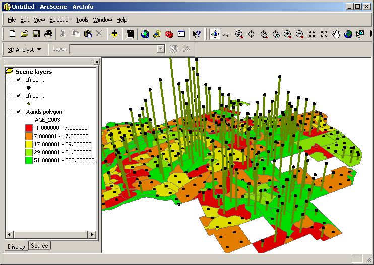
Most of the images described in this section are surface drapes. In this 3D scene, the CFI plots are not draped over a surface, so the background appears flat. CFI plot centers are shown twice, once as black points offset at a value proportionate to wood volume, and again as extruded lines at the height proportionate to the wood volume attribute. Also displayed are the forest stands in a graduated color symbology based on stand age (young = red; old = green).

Navigation and moving around in real-time

It is easy to move around a 3D scene. Fast computers with good video cards will be able to draw and respond more rapidly to navigational control.

The Navigation tool is the controller for rotation, panning, zooming, and altering the orientation of the surface. Using this tool in combination with keyboard keys and different mouse keys controls its behavior (see help on navigating the 3D Scene).

When the cursor is in the display area, during rotation, panning, or zooming, stopping the motion of the mouse stops the motion of the surface in the scene. To have the motion continue, move the cursor outside the viewer while keeping the mouse button pressed. Small movements of the mouse outside the viewer will initiate movement and allow it to continue.

Contouring

Contouring is covered in Raster Analysis II. In addition to creating entire contour data sets, with the 3D Analyst it is also possible to create single contours as simple graphics using the Contour tool .

Line of Sight, Visibility Analysis, and Surface Profiling

The Spatial Analyst Extension includes a few functions for line of sight and visibility analysis.

The Line of Sight tool , which analyzes the visibility of a line drawn between two points. Locations of the landscape that are visible along the line between the observer and target are shown in green, and locations that are not visible are shown in red.

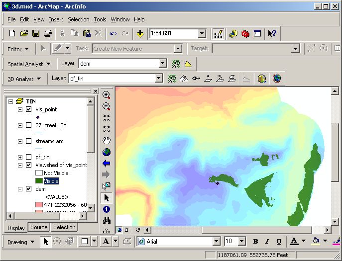
The Surface > Calculate Viewshed menu choice is used to determine what parts of the landscape are visible from a given point. This generates a grid which shows all areas that are visible, rather than simply what places are visible along a line between a target and observer. Here, all areas that are visible are green.

For 3D lines drawn on a data frame, or for features selected from line feature classes, it is also possible to create surface profiles based on underlying surface data using the Create Profile Graph tool .

Color hillshade mapping

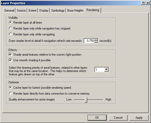
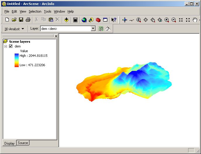
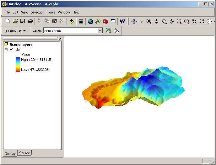
The 3D Analyst includes powerful tools for visualizing landscapes. One of the most powerful is color hillshading. This displays elevation in user-defined colors, such as green > yellow > red color ramps, but also applies analytical hillshading to the view. This creates a visual model of the landscape in which features appear to have volume. Compare the two 3D scenes, one with analytical hillshading and one without:

The option for shading is specified by the check box in the Layer Properties > Rendering dialog.

Steepest descent

The watershed delineation tools used in the section on Hydrologic Modeling allows the creation of catchment areas. For any point within a watershed, it is known where the ultimate outlet point is. But where does the actual water flow across the surface? With a surface model loaded in a data frame, the Steepest Path tool becomes available. When a point is clicked on the data frame, a graphical line is added to the data frame, following the path of steepest descent.

This graphical object can be copied and pasted in a new shapefile and added to a 3D scene.

Slope and aspect calculation

Many physical processes and management objectives are related to slope and aspect. Slope is defined as the (change in elevation / change in planimetric distance). Sometimes slope is defined in degree measure, and sometimes in percent measure. Aspect is the compass direction of the slope, facing downhill.

For TIN surface models, slope and aspect are automatically calculated as attributes of each triangle. However, for elevation grids, slope and aspect are not native attributes. It is easy to calculate slope and aspect for elevation grids, using the Surface > Derive Aspect and Surface > Derive Slope menu choices.

ArcGIS calculates slope in degrees, which can be converted to percent slope by multiplying the tangent of the slope (measured in radians) by 100%.

Here is a data frame containing a slope grid. Notice that the steepest slopes are located in the valleys and canyons of the Mashel and Nisqually rivers.

Aspect classes are shown here. Note how aspect changes abruptly at stream channels and ridgelines.

Return to top | Ahead to Help Topics

Syllabus Schedule Class Meetings Assignments Course Data Contact Us CFR 520 Lab Locations Software Collect It Page

The University of Washington Spatial Technology, GIS, and Remote Sensing Page is supported by the School of Forest Resources

School of Forest Resources