Introduction to Geographic Information Systems in Forest Resources

UW Home GIS@UW Search

Syllabus Schedule Class Meetings Assignments Course Data Contact Us CFR 520 Lab Locations Software Collect It Page

Objectives:

• to become familiar with a few more common analytical functions (more analytical functions on raster surfaces models will be dealt with in 3-D and Surface Modeling).

1. Perform drive substitution to create drives L (CD) and M (removable drive).
2. Open a new map document
3. Importing data from generic raster files
4. Getting and importing 10 m USGS DEMs
5. Mosaicking grids
6. Mapping contours
7. Calculating distance surfaces and buffers
8. Calculating summary attributes for features using a grid layer ("Zonal statistics")
9. Cross tabulating areas
10. Reclassify a raster grid layer
11. Calculating neighborhood statistics

Perform drive substitution

Perform drive substitution to create the virtual drives L and M.

1. If you need to, enable the Spatial Analyst extension and dock the Spatial Analyst toolbar in your ArcMap application window.
   
   
2. Delete everything you can from your removable drive.
   
   
3. Create a directory called M:\r_an_2 to hold today's work.
   
   
4. Create a new map document called M:\r_an_2\r_an_2.mxd.
   
   
5. Set the working directory to this location as well (Geoprocessing > Environment > Working Directory).
   
   
6. Make sure to save early and often during this exercise.

1. Download the file q1822.zip, and save it in M:\. (The full set of Washington State DEMs is available from a server in Geological Sciences.)
   
   
2. Unzip the file, placing the unzipped file (q1822.dem) in M:\.
   
   
   1. If you are curious about the structure of the file, open a command prompt and use the command
      
      more M:\q1822.dem
      
      
      
      This shows the file represents the Eatonville, WA quadrangle, the data source was high-altitude photography (HAP) flown on August 6, 1981. The cell size is 30 m. The large numeric values are are header values for grid XY origin, rotation, etc. The smaller values are elevation in meters.
      
      
   2. Use the <SPACE> key to continue looking at values. Use the <Q> key to stop looking at the file.
      
      
3. The extracted file is a USGS format digital elevation model (DEM) for the USGS 7.5' topographic quadrangle of Eatonville, WA. The DEM is a raster dataset representing elevation values.
   
   
4. Create a new data frame and rename it to Eatonville.
   
   
5. The USGS-format DEM cannot be added directly to ArcMap, but needs to be imported to grid format first.
   
   
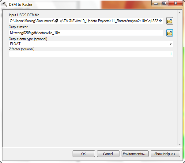
6. Open ArcToolbox and search for the tool containing the word dem:
   
   
   
   
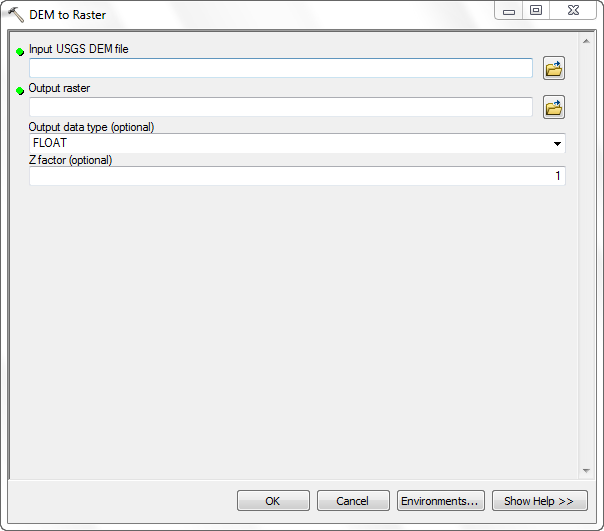
7. Open the tool.
   
   
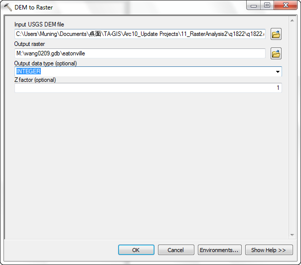
   1. Set the Input USGS DEM file to the unzipped dem.
      
      
   2. Set the Output raster to a grid called M:\NETID.gdb\eatonville or M:\r_an_2\eatonville
      
      
   3. Change the Output data type to INTEGER. These USGS DEMs are stored in integer meters, so storing the grid as integer is appropriate.
      
      
      
      
   4. The new layer will be added to the data frame.
      
      
      
      
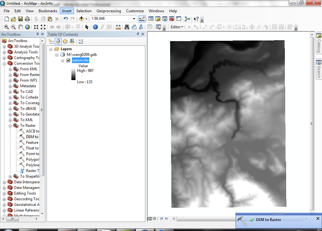
   5. Alter the color ramp (you can do this quickly by clicking on the existing color ramp in the table of contents):
      
      
      
      

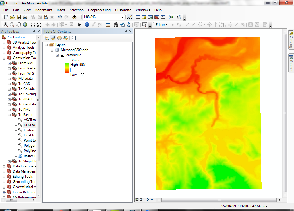
You have just successfully downloaded a public-domain digital elevation model, imported it into ArcGIS, and displayed it in a stretched color ramp by elevation. Almost all of the DEMs for the US are available for free download. DEMs are used in all aspects of GIS analysis of landscapes. Elevation is one of the most basic things we need to know about landscapes. Also, elevation datasets are the basis of slope and aspect datasets, and will be used for developing watershed delineations.

Harvey Greenberg runs a server in Earth & Space Sciences that maintains a large number of data sets for Washington state, including 10 m DEMs (the ones you just used are 30 m).

1. Create a directory called 10m to hold the 10-meter DEMs in your M:\r_an_2.
   
   
2. Right click on the link to the left and "Open in New Window". http://gis.ess.washington.edu/data/raster/tenmeter/byquad/index.html
   
   
3. The Washington 10 m DEMs page should open.
   
   
   
   
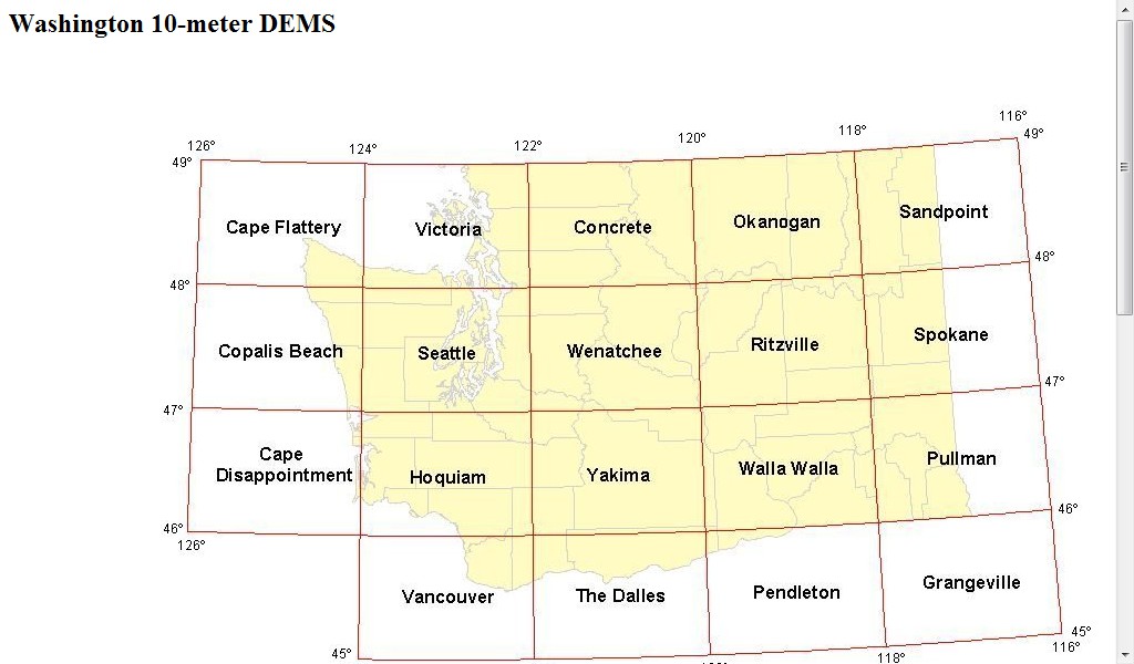
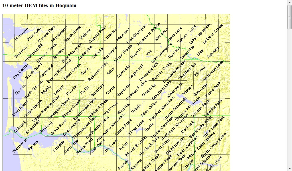
4. Pack Forest is in the Hoquiam quad, so click inside the Hoquiam 1° quad.
   
   
5. Click on Eatonville 7.5' quad and save the file to the new directory. Do the same for Elbe.
   
   
   
   
6. Unzip the files.
   
   
7. Import these DEMs using the same method as before, but import as floating point (select FLOAT as the Output data type). Even though the values in the DEM file are stored as decimeters, ArcGIS will automatically apply the scaling factor to create a grid with meter values.
   
   
   
   
8. Change the symbology of the grids to Classified rather than Stretched (use default colors and class assignments), and zoom in until you can see individual cells. You should be able to clearly see the difference not only in cell size but in the level of detail between the 10 and 30 m DEMs.
   
   10 m
   
   30 m
   
   
9. Note also the difference in file sizes. The 10 m DEM will take up more disk space for two reasons (the 1/3 smaller cell size means 9 times more cells to store for the same area coverage, and floating-point values take up more storage space than integer values).
   
   10m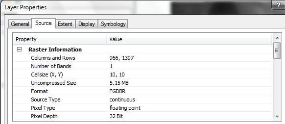
   
   30m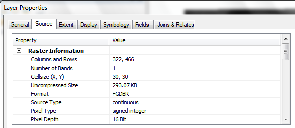
   
   
10. Remove the 10 m grids from the data frame.

Merging adjacent grids ("mosaicking")

Mosaicking will create a single seamless grid and also smooth the transition between grids by performing an averaging function near the edge.

1. Using the same method as above, download, import, and unzip the Elbe, WA 30 m DEM (q1823.dem). Call the output grid elbe.
   
   
   Even if you use a similar color ramp, you can still see the hard edge between the two grids. You can also see that these are still two separate grids in the data frame's table of contents.
   
   Here is a zoomed view with a classified rather than stretched symbology.
   
   
   
   
2. Use the Identify tool to identify a few cells on either side of the edge between the grids (use <CTRL> to identify multiple locations, and make sure to identify from Visible layers.
   
   For these cells on the edge, the elevation difference is 9 meters.
   
   
   
   
3. Open the Mosaic to New Raster (ArcToolbox\Data Management Tools\Raster\ from the ArcToolbox) and put these two layers as the input. Select the proper file name as the output. [Number of Bands: 1]
   
   
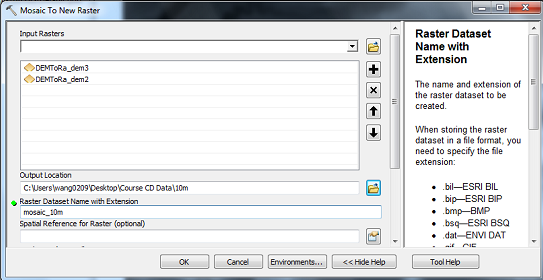
   This tool will "create a new raster layer by mosaicking the Eatonville grid with the Elbe grid."
   
   
4. After a few moments you will see the result as Calculation in the data frame.
   
   
   
   Zoomed to full extent:
   
   
   
   
5. You will see that there is a smooth transition between the two source grids in the output. Use the Identify tool again to investigate cell values. Note how the new grid has taken on the values from the source grids.
   
   

You have just downloaded, imported, and merged two adjacent USGS digital elevation models. If your study area runs across several USGS quad sheet boundaries and you need to perform analysis using elevation data, you will need to mosaic them together.

Mapping contours

1. Go back to the Eatonville data frame.
   
   
2. From the Spatial Analyst Tool, select Surface > Contour.
   
   
   1. Set the contour interval to 10 m.
   2. Place the output as a shapefile called Contour_10m.
      
      
      
      
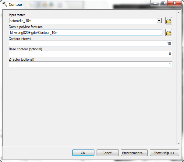
3. After a few moments, the process will finish, and a new line layer will be added to the data frame.
   
   
4. Zoom in so that you can see the contour lines clearly.
   
   
   
   
   
   
5. Using the Selection tool, select a single contour line. Open the attribute table and click the Selected button.
   You will see that the record for the selected contour contains the value of the elevation of that selected line.
   
   
   
   
6. How do you think these lines compare to the contour lines in the Pack Forest data set?
   
   
   
   
   

You have just created an entire vector contour line layer. Use this technique to create contour line data if you only have available raster elevation data, but need contours on your map. Beware, however, that the contour lines are only as good as the input data, which in many cases, are not very good at all. There are also issues of line generalization that may affect data quality.

Calculating distance surfaces

1. Create a new data frame called Pack Forest.
   
   
2. Add the streams layer from the L:\packgis\packgis.mdb.
   
   
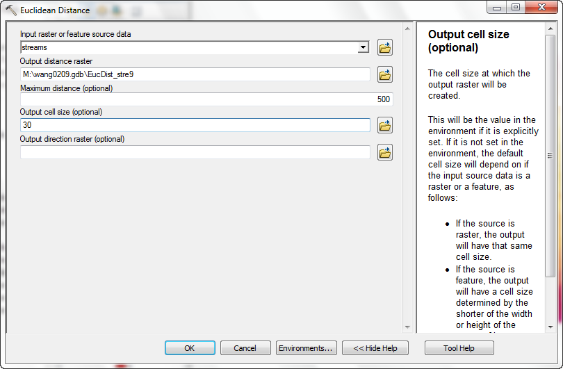
3. From the Spatial Analyst Tools menu, select Distance > Euclidean Distance. Use a cell size of 30.
   <Note> Do not save this file into Geodatabase or it may cause some errors.
   
   
   
   
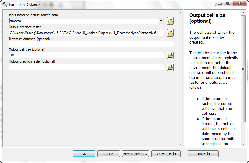
4. The new grid layer: streambuf will be added to the data frame.
   .
   
   
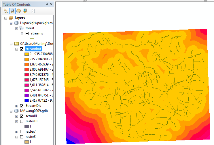
   Now every cell in the output grid has a value for its distance to the closest stream. This has a similar look as a buffer with concentric buffer zones, but rather than quantized distance zones, each cell is coded for its own distance to the closest stream rather than simply being coded for "inside or outside" a buffer with a particular range of distance values.
   
   
5. Using the Identify tool, examine a few values for the new grid, starting on one of the stream lines and then moving outward.
   
   
   

Do you see how this is different from the buffer function in the vector world?

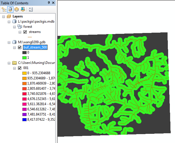
Create buffers

Now that you have a surface which has distance to each stream, create a grid layer which represents the cells within 500 ft of existing streams.

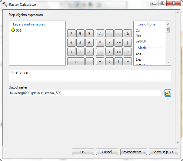
1. From the Spatial Analyst Tools\Map Algeba, select Raster Calculator.
   
   
2. Format a calculation that only takes cells within 500 ft of streams (File 001 is the buffered layer).
   
   
   
   
   
   
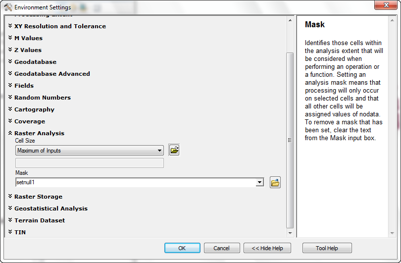
3. To create a mask grid containing valid cells within the 500-ft distance, perform another Raster Calculation using the setnull map algebra function:
   
   setnull ("Calculation" == 0, 1)
   
   
   
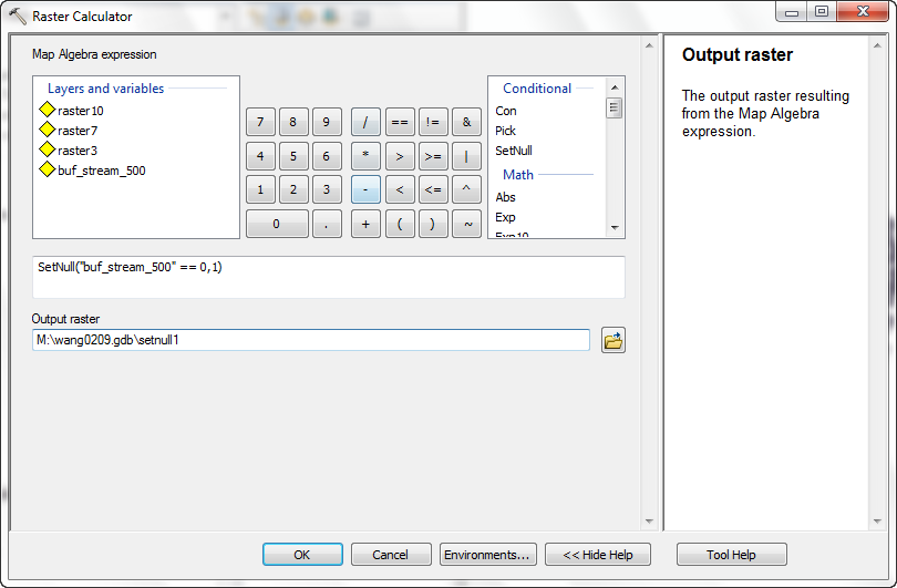
   This expression means "for each cell, if the value of buf_stream_500 is equal to 0, make the output value no data, otherwise make the output value 1."
   
   
   
   
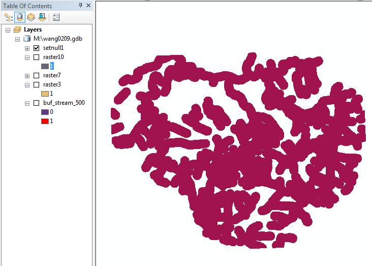
4. Now set Analysis Properties for Analysis masking, and use this setnull1 layer as the mask grid (Environments>Raster Analysis):
   
   
   
   
5. Use the Raster Calculator to create a new layer with the expression
   
   "Streambuf"
   
   
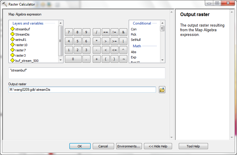
   This will create a new grid that is identical to the original distance grid, but its will have value for cells only within the mask grid. The mask limits the spatial extent of output cells.
   
   
   
   
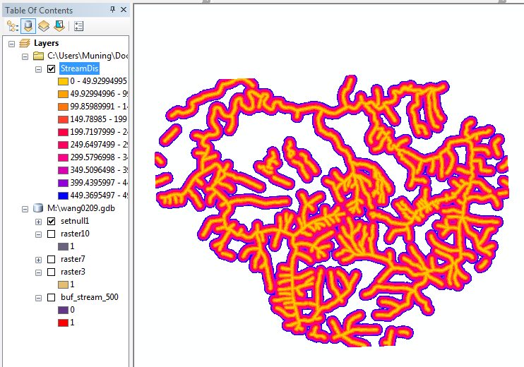
6. You should be able to verify that the new grid has value only for cells within the mask grid by using the Identify tool. When you click within a buffer zone, you will get the distance of that cell to the closest stream. If you click outside of the 500 ft buffer, there will be no cell value reported in the Identify Results dialog.
   
   
   
   
7. Delete any layer from the Mask setting in the Environments.
   
   

The other method to limit the distance is:

1. Perform the same Distance calculation as before, but enter the Maximum distance of 500 ft:
   
   
   
   
   
   Although this method is easier, you will find that many grid operations do not include cutoff values, and you may need to use multi-step processes in order to perform analyses that are limited in spatial extent by a mask grid

You have just created a distance surface grid from a stream vector layer. These distance surfaces are similar to buffers, but rather than having a simple binary in-or-out value, the cells are coded with the actual distance of the cell center to the nearest stream. If you are performing some kind of modeling where the actual distance from a feature (rather than an inside/outside a buffer) is important, you can use this technique. For example, salamanders are more likely to be found closer to stream channels.

Calculating summary attributes for features using a grid layer ("Zonal statistics")

Zonal statistics are used when you have a zone data set (source can be either a grid or vector data set) and want to know summary statistics for an underlying grid.

1. Create a new data frame and add the grid layer dem and the polygon layer stands from the L:\packgis\packgis.mdb.
   
   
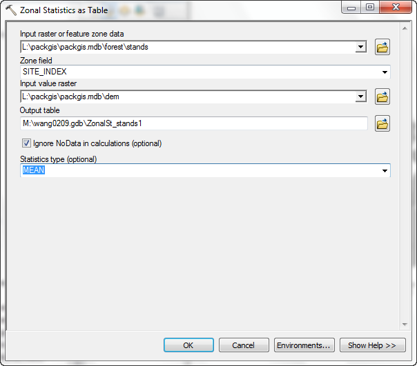
2. Select Spatial Analyst Tools > Zonal > Zonal Statistics.
   
   
   1. Choose stands polygon as the Zone dataset.
   2. Select the item SITE_INDEX as the zone field. This specifies that we are interested in grouping the stands together and analyzing by unique value of site index.
   3. Select dem as the Value raster.
   4. Select Mean as the Chart statistic.
   5. Put the output table in M:\NETID.gdb\ZonalSt_stands1.
      
      
      
      
3. The zone summary will take a few moments. What is happening here? The raster processor takes every elevation cell that overlaps with each stand polygon and creates summary statistics based on stand groupings. For example, the cells that overlap with all stand polygons with a site index of 100 are extracted, and the mean elevation value is calculated for that group of cells. Finally, a summary table will be created.
   
   
   
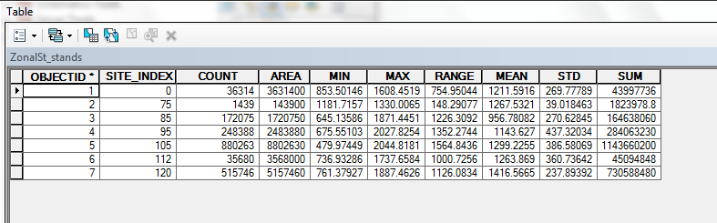
   This table contains the statistics for the Dem grid (elevation) for each Site Index zone in Stands.

Area cross-tabulation is useful for comparing different datasets for the same area, as well as for comparing the same data layers at different times.

A raster approximation of the vector intersect

1. Create a new data frame called XTab.
   
   
2. Add the stands and soils layers from L:\packgis\forest folder to the data frame. Since we do not have existing raster layer for this exercise, we would like you to make two layer from stand and soil.
   
   
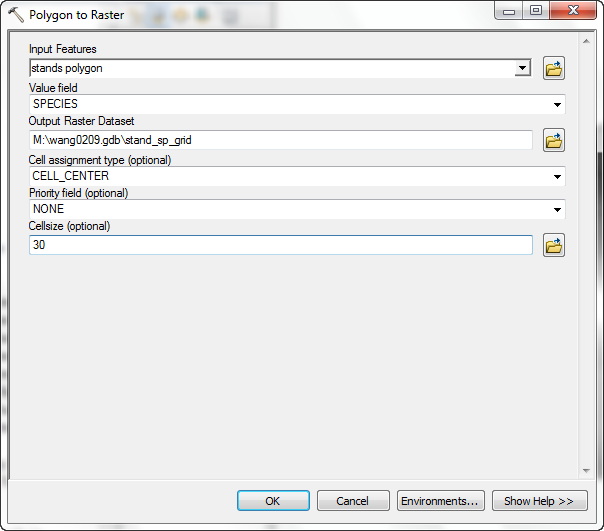
3. Convert the stands feature class to a raster (ArcToolbox > Conversion Tools > To Raster > Polygon To Raster).
   1. Convert based on the SPECIES field.
   2. Place the output data set in M:\NETID.gdb\stand_sp_grid.
   3. Use a cell size of 30 m.
      
      
      
      
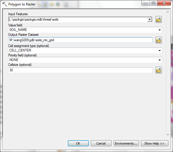
4. Perform a similar conversion for the soils layer (but use SOIL_NAME as the conversion field):
   
   
   
   
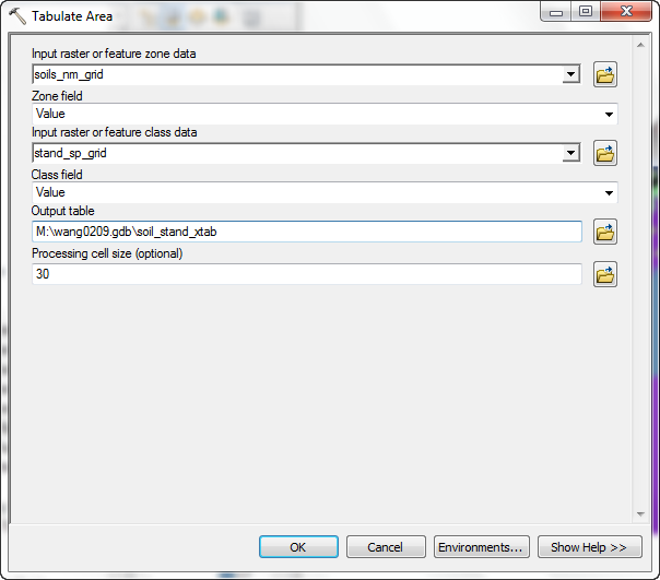
5. Search for the term tabulate in ArcToolbox to find the area cross-tabulation tool. After it is found, open the tool.
   1. The first input layer is the soil grid
   2. The second input layer is the stand grid.
   3. Place the output table in M:\NETID.gdb\soil_stand_xtab.
   4. Click OK.
      
      
      
   5. Open the table (you may need to click the Source tab in the table of contents). The output table has 12 records (corresponding to the intersected area only include 12 of 25 soil names; as you can see if you open the table for the soil grid). The VALUE field represents the values from the soil grid table. The other fields represent the values from the stand grid.
      
      
      
      
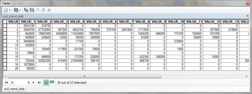
   6. The value 1-18 is stand_species_ID from 1-18. Each value here is counts. For example, the count that intersect soil name 1 and stand_species 1 is 2933100, which equals to 2933100*30*30 square feet. Tabulated Area is only used to get the intersected area between two raster layers. Can you think of how this could be done using vector overlay?

Sometimes it makes more sense to work with reclassified data rather than raw continuous data. For example, there may be specific elevation ranges in which you might find different vegetation types. In order to model vegetation distribution it might be better to have an elevation class grid rather than one containing raw continuous elevations. Reclassifying your data is similar to changing the classification in the legend for a layer, but rather than just altering symbology, it creates a new grid data set with these values.

1. Close the Properties.
   
   
2. Select Spatial Analyst Tools\Reclass\Reclassify from the ArcToolbox. Select dem as the Input raster. The default method for classification is a 9-class manual break-down, where the class breaks are automatically selected. <Note: Remember to check the right geodatabase to save raster layers>
   
   
   
   
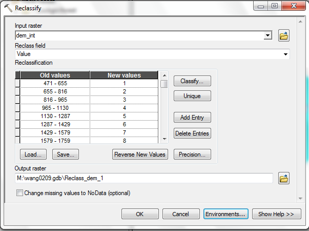
3. It is possible to manually reclassify your data, but this can be inefficient if you have a large number of classes and values. Instead, we will build a remap table.
   
   
4. Open Excel and create a spreadsheet formatted like so:
   
   
   
   Use Excel's auto-fill function to make this a breeze (ask your local Excel guru or ask the instructor for a demonstration if you don't know how to do this, or look it up in Excel help). Each record in the table defines the range and output values. For example, the first record will take input cells with values from 400-500 and remap them to a value of 500 in the output.
   
   
5. Save the file office 97-2003 file format and import into your geodatabase
   
   
   
   
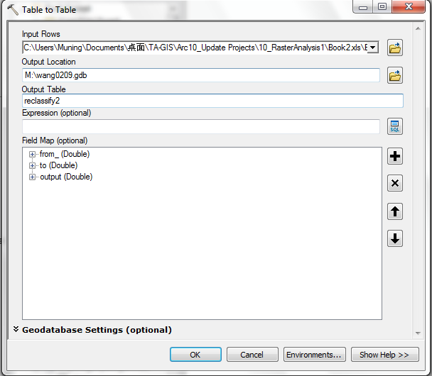
6. Make sure to close the spreadsheet or there will be a sharing violation between ArcGIS and Excel. Make sure every field has the right value after you import your data.
   
   
7. Add the table from Geodatabase, add a field called "output" and select short integer as the data type.
   Use the field calculator and type in "Output"=[out].
   
   
8. Click Spatial Analyst Tools\Reclass\Reclassify by Table
   
   
   
   
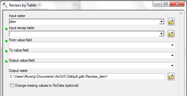
9. The default location for the output grid is the default geodatbase, meaning the output will be placed in the working directory. With this setting, place the raster dataset on your M:\NETID.gdb\dem_reclass_100. (The Output value field may encounter some error message at first place, please try to select the correct value twice to get it worked.)
   
   
   
   
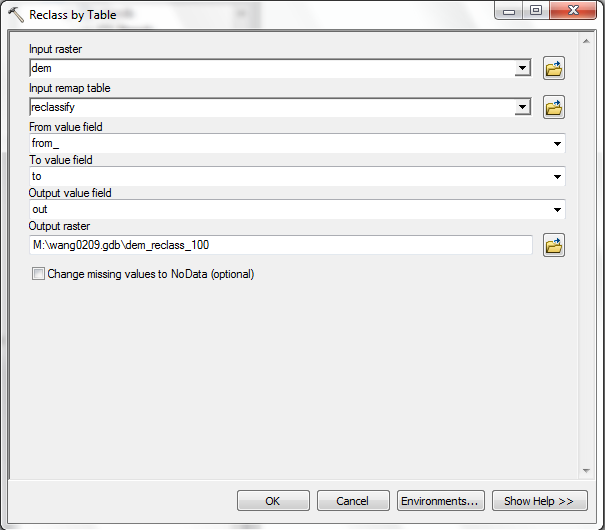
10. Click OK.If there is a error indicates a limitation in the length of names for raster grid datasets. Alter the name to dem_rcls_100, then click OK.
    
    
11. Now you see the new grid with reclassified values.
    
    
    
    
12. Open the table for the new data set. You can see how the large number of values from the original elevations have been collapsed into classes.
    
    
    

Reclassification of a raster grid layer assigns new output values to groups of input cells. In this case, we created a new raster grid from the selected set of the Dem_int raster grid layer. Reclassification is a technique that can make data more understandable, but always includes a loss of original information (the original values are lost). The other problem with reclassification is that the resultant raster grid attribute table does not have descriptive values, only class numbers. Reclassify is also a local function, because it assigns new cell values for each cell independently of other cells.

What parts of the forest has the greatest topographic complexity? Based on a 5 by 5 cell kernel passed over the entire landscape, calculate the standard deviation of elevation within that 5 by 5 cell kernel, and place the output of each of those calculations in the center cell of the output grid.

1. From the Spatial Analyst Tools\Neighborhood, select Block Statistics.
   
   
   1. Select dem as the input data set
   2. Select the statistic Standard Deviation.
   3. Use a 5 by 5 rectangle of cells.
   4. Set the output cell size of 10 from the Environments\Raster Analysis.
      <Note> This file can not be stored in the geodatbase, save to your removable drive instead
      
      
      
      
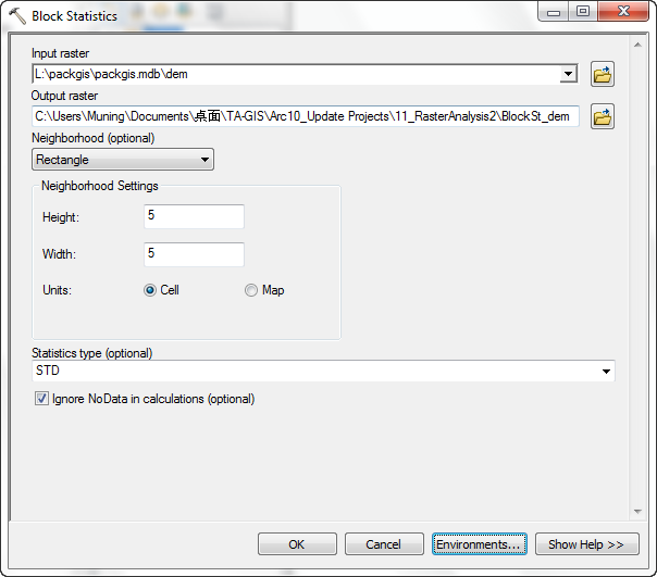
2. After a few moments, a new grid layer will be added, called BlockSt_dem1 ("neighborhood standard deviation of Dem").
   The values for each cell of this grid layer represent the standard deviation of elevation in a 5 by 5 cell neighborhood for each original cell in the Dem grid. The standard deviation in this case gives a measure of the local variability in elevation.
   
   
   
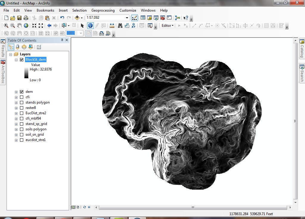
   The darker areas are similar in location to the places with high slope for Pack Forest. This is no coincidence; places with the greatest slope over a small area will have the greatest variability in elevation over the same area.
   

The same basic technique could be used, for example, to characterize land use or land cover types. For nominal data such as land use or land cover, the neighborhood statistic Variety would render a new grid layer in which the output cells represent the number of distinct classes within the kernel area.

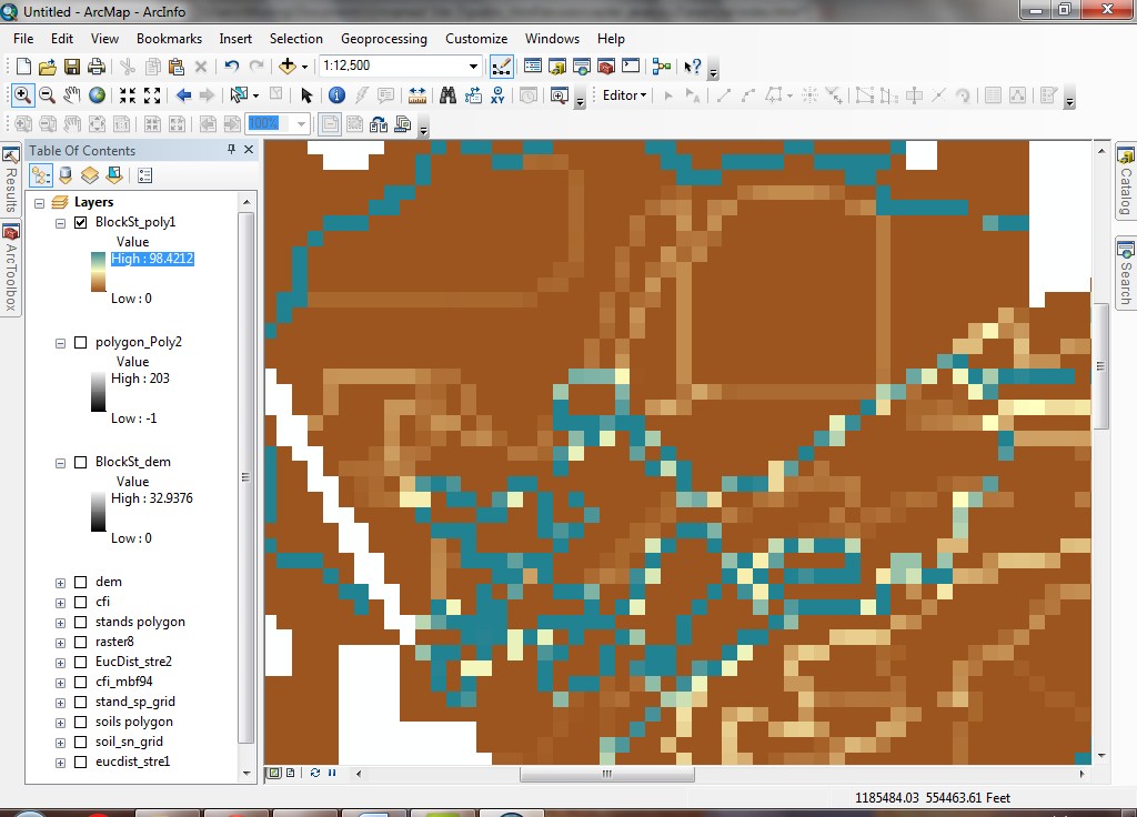
Here is an example of a neighborhood calculation based on stand ages. The forest stands have been converted to a grid based on the stand age (Age_2003) values. The highest-contrast edges (those that have the greatest difference in age) result in cells with a higher standard deviation value (shown in a darker shade of purple). Can you reproduce something like this using the Pack Forest stand polygons, based on the Site_index field values?

REMEMBER TO TAKE YOUR CD AND REMOVABLE DRIVE WITH YOU!!!!

Return to top

Syllabus Schedule Class Meetings Assignments Course Data Contact Us CFR 520 Lab Locations Software Collect It Page

The University of Washington Spatial Technology, GIS, and Remote Sensing Page is supported by the School of Forest Resources

School of Forest Resources