
Introduction to Geographic Information
Systems in Forest Resources |
Exercise:
An ArcGIS Sampler
Objective:
- Become familiar with ArcGIS 's basic functionality and user interface.
- Perform drive
substitution to create drives L (CD) and M (removable drive). Note: ignore this drive substitution step if this is your first lesson.
- Identify the CD and removable drive letters
- Download a few files
- Start ArcGIS
- Switch active data frames
- Alter drawing properties
- Identify features
- Measure distances and areas
- Get information about features
- Display and modify a table
- Display and modify a graph
- Create a layout
- Close the project
Perform drive substitution
Perform drive
substitution to create the virtual drives L and M.
Identify the CD and removable drive letters
- Put the course CD in the CD drive.
- Plug your removable drive into the USB port on the PC.
- Click "Computer" from the Main Menu. The removable and CD drives should show up in the file manager like below but you will see Drive L (for CD) and M (for removable drive).
One of these removable disks should be your removable drive. The course CD
will show up with the name esrm_250 or similar names.
- Make a note of the drive letters. You should always be aware of which drive
letters are which as you move from machine to machine.
Download a few files
These files will be used a short time later in the exercise.
Start ArcGIS
- The location of the ArcMap shortcut may vary from system to system. It should
be in a path similar to this:
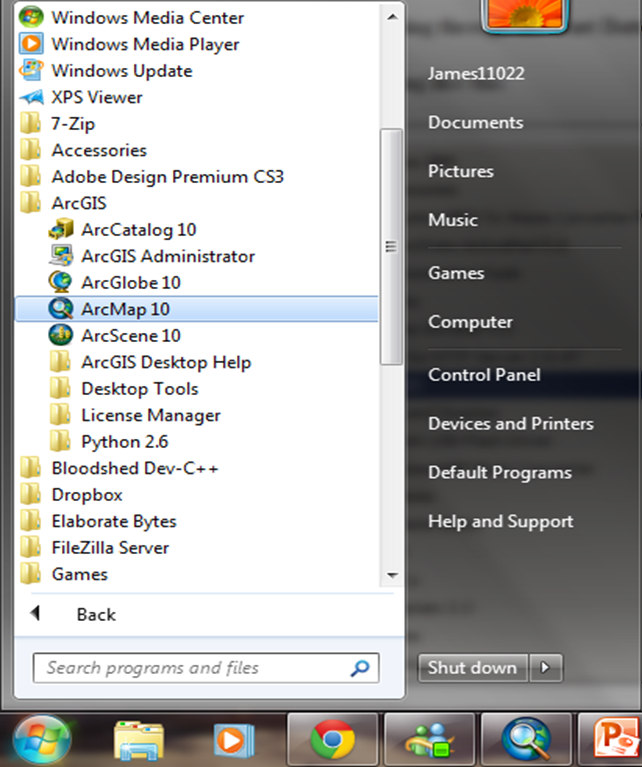
During the first lab session, you will be shown where the ArcGIS shortcut
is on the computers in the lab.
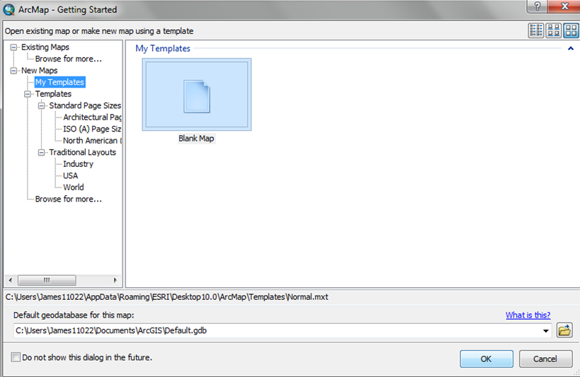
- When ArcMap opens, a dialog may open with choices for what to do next. Click
the radio button for A new empty map or close the dialog.
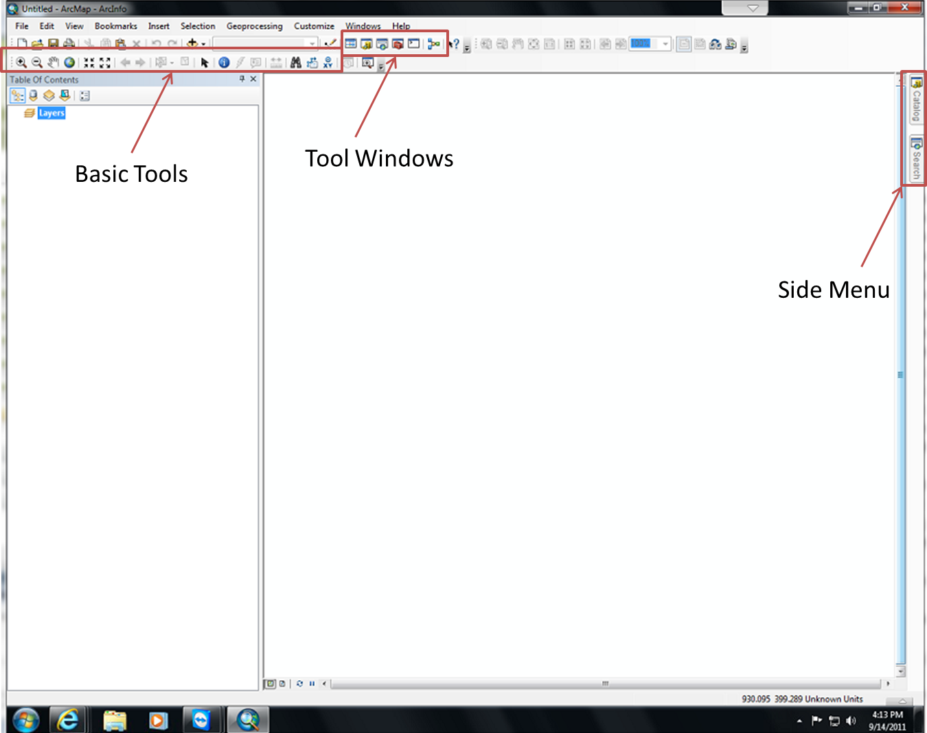
The project will open with a single window containing a few menu choices, a few toolbars icons, and a few
buttons. In this windows, you can see the basic tools, several tool windows, and the side menu at the same page.
Open the Sample Project
Make sure that the data CD is in the CD drive, and your removable drive
is connected.
- Important !!!!!!!! Follow the instructions
for substituting drive letters before attempting to open the map document.
Note that each time you work in this class, you should follow the drive substitution
instructions! !!!!!!!
- Download the arcgis_sampler.mxd file
and save it in the main directory of your removable drive. (Note:
make sure the file you downloaded has the name arcgis_sampler.mxd.
Web servers and browsers can arbitrarily rename files. If the file has a different
name, rename it to the correct name.)
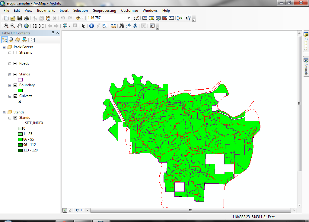
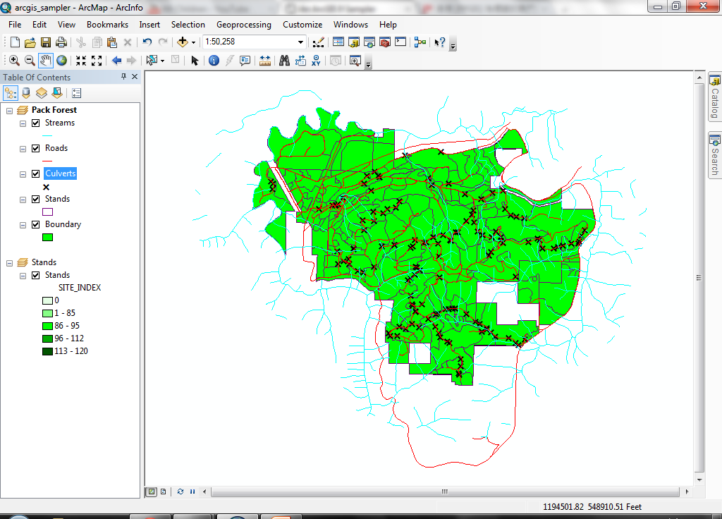
- From the File menu, select Open and navigate to the location
where you downloaded the arcgis_sampler.mxd file. It will open and
automatically load datasets from the CD. You will see the table of contents
on the left. On the right side, you will see a data frame containing
several different features.
- Save the project with your initials so you will be able to start over if
necessary. From the File menu, select Save As and name the file
with your initials (my file will be called arcgis_sampler_pmh.mxd).
Switch active data frames
A single map document may have more than one data frame. A data frame contains
a number of layers with similar thematic properties and covering the same area
of ground. When the map document opens, you will notice that the Pack Forest
data frame is active (it is printed in bold text). It is possible to switch
between active data frames
- Right-click on the Stands data frame title
 and select Activate.
- You will see how the display changes.
- Right-click back on the Pack Forest data frame title and select Activate.
Note how the display changes back to the way it was before.
Summary: You have just learned to switch active data frames. Typically,
a single map document will only contain references to data sources that have
some reason to be included as a group. Likewise, a single data frame should
only contain layers that have something to do with each other.
Alter drawing properties
- The project opens with a map of Pack Forest. Notice that there are several
layers (in this case, Streams, Roads, Stands,
Boundary, Culverts) in the view document. Also note that streams
do not display, since the layer is not checked "on."
- Click on checkbox to the left of the Streams layer in the Table
of Contents to display the layer.
- Now that all layers are turned on, notice that the points for the layer
Culverts is not displayed. This is because layers draw in order, from
bottom to top of the list of layers in the Table of Contents. Click on the
Culverts layer name and holding the mouse button down, drag it up the
list (above Stands). Now the points representing culverts should be
visible.
If you have layers loaded in a view and some do not appear visible as you
think they should, check the drawing order.
- Many of the Culverts are spaced so closely together that they are not discernible
from each other at this scale. In order increase the scale to see the individual
Culverts, click the Zoom In tool
 . The pointer will change to a magnifying
glass
. The pointer will change to a magnifying
glass  when placed
over the map display.
when placed
over the map display.
Note that the cursor will always change to match the type of tool used. When
you become familiar with ArcGIS, you will be able to tell which tool is active
by just looking at the cursor.
- Click and drag a rectangle (click the mouse button down at one corner of
a rectangle, and drag to the opposite corner, then release the mouse button)
near the center of Pack Forest. Now you will see the individual culverts when
the map redraws at the new scale.
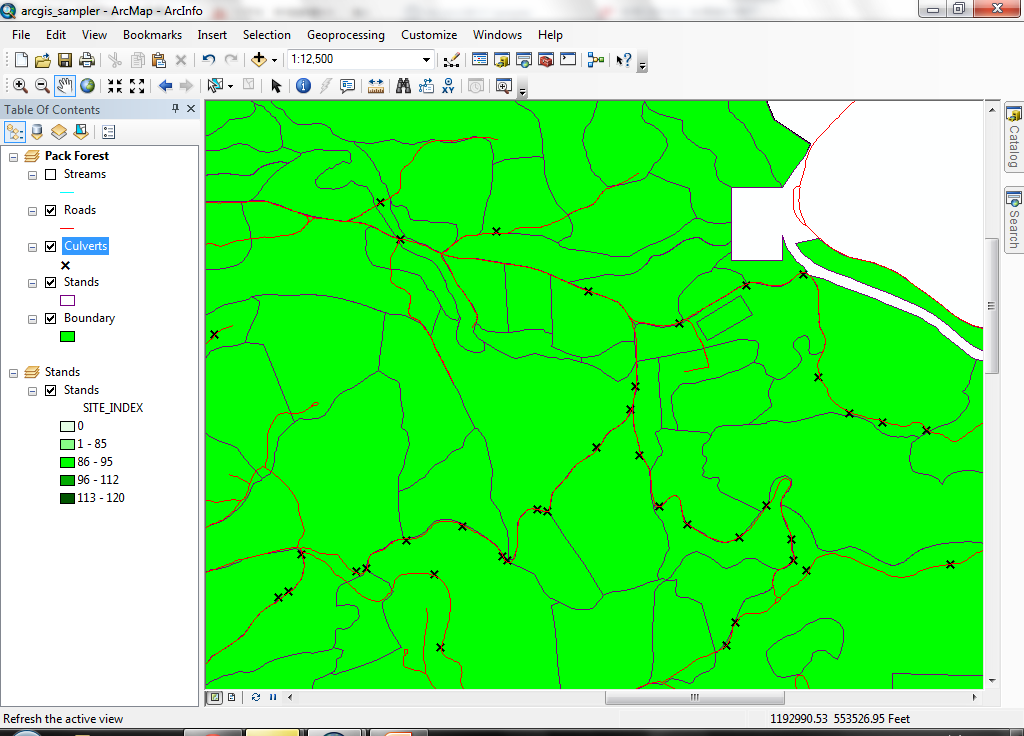
Now you can see the individual culverts, roads, and streams.
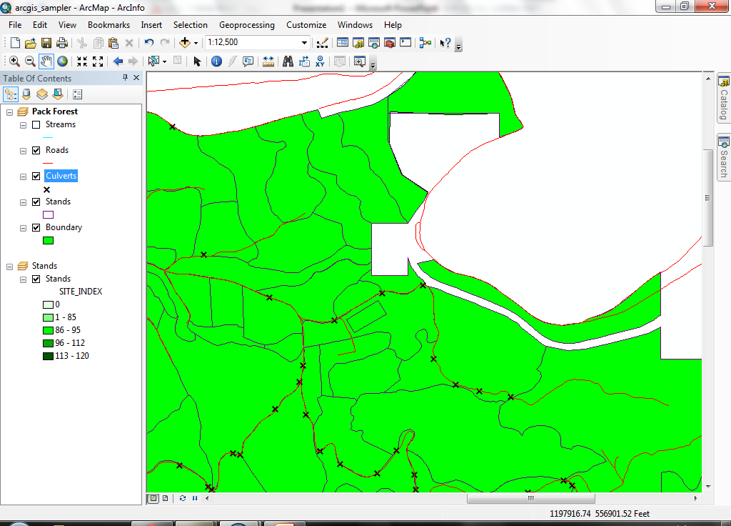
- Click the the Pan tool
 . Place the cursor
on the map view, then click and drag in any direction. When you release the
mouse button, the view will redraw in its new position. You can use this to
move to a different area of interest without zooming out and back in. A lot
of time is wasted by zooming in and out unnecessarily, because after each
zoom, the view needs to completely redraw.
. Place the cursor
on the map view, then click and drag in any direction. When you release the
mouse button, the view will redraw in its new position. You can use this to
move to a different area of interest without zooming out and back in. A lot
of time is wasted by zooming in and out unnecessarily, because after each
zoom, the view needs to completely redraw.
- There are several buttons and tools on the Tools toolbar for controlling
map extent. You have just used the Zoom in and Pan tools. Now
examine the zoom buttons:


In order from left to right, these perform
- zoom out (tool)
- zoom in (tool)
- fixed step zoom in (button)
- fixed step zoom out (button)
- pan (tool)
- go to previous extent (button)
- go to next extent (button)
- zoom to full extent of all layers (button)
- Right-click the layer name for Culverts and select Zoom to layer,
and you will zoom to the full extent of the Culverts layer.
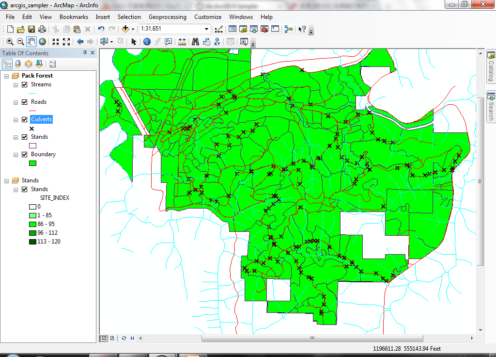
All the culverts are visible, but the rest of the view is truncated.
- Now click the Zoom to full extent button
and the view will zoom to contain the full extent of all layers. If you have
several datasets that represent the same area of the earth, but not all the
datasets display as you think they should, zooming to full extent can show
you if the datasets were built with the same spatial referencing framework.
- Click the Zoom to previous extent button
a few times to see how you can return to a previous display extent. .
- Experiment with the Fixed zoom in
and Fixed zoom out
buttons to see how they are used.
Summary: You have learned to turn layers on and off, to alter drawing
order, and to navigate around the view by zooming and panning. The more layers
you have displayed, and the more complex those layers, the longer it will take
to draw your view. For this reason, you should get very familiar with these
zooming tools and buttons so that you can work efficiently.
Identify Features
- To find out some cursory information we will perform an identify.
- Click the Identify tool
 in the tool bar.
Move the cursor onto the map display of the view. You will see the cursor
change from the pointer to the Identify cursor
in the tool bar.
Move the cursor onto the map display of the view. You will see the cursor
change from the pointer to the Identify cursor  . The active
area of the identify cursor is a 3-by-3 pixel window centered at the end of
the pointer.
. The active
area of the identify cursor is a 3-by-3 pixel window centered at the end of
the pointer.
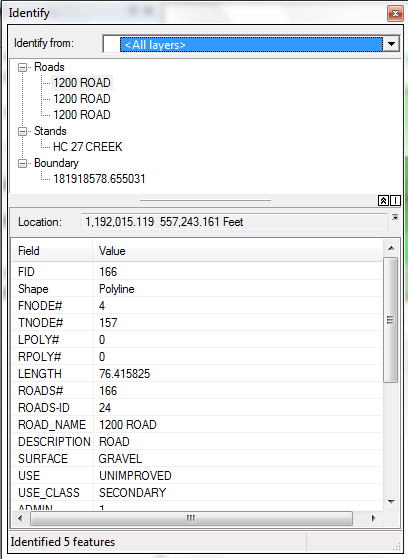
- Click on one of the forest stand polygons. The Identify Results dialog
will appear, listing the attributes of the stand you just selected. Keep the
<CTRL> key pressed and click on a few more stands, and each successive
stand will be added to the identify results window. You can click up and down
in the Identify Results dialog to view attributes of already identified
features.
Using the identify tool is a good way to get a brief look at the attribute
values for a selection of features in your spatial datasets.
- Note the dropdown list for Layers. There is some control over which
layers are identifiable. Use help to explain what these choices mean.
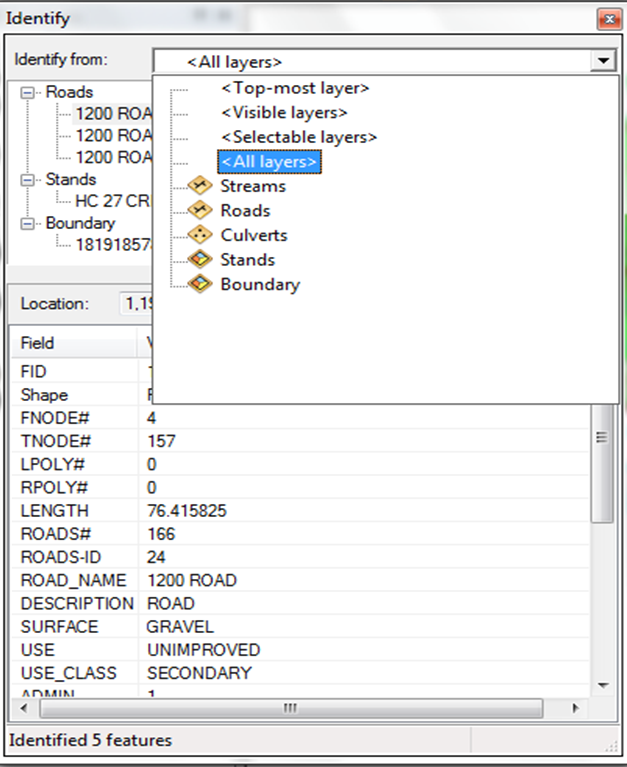
- Turn off a few layers and change the dropdown to <Visible layers>.
.
- Perform another Identify where several features overlap. What do
you see in the Identify Results dialog?
- Keep the dialog open for the next step.
Summary: You have use the Identify tool to browse attributes for individual
features. Use this whenever you are curious about the type of data you have,
and what those datasets represent. If you are interested in the attributes of
features at a particular location, Identify is the right tool for the job.
Note: the active area of the identify pointer is a 3-by-3 pixel window. Any
features that fall within this window will be identified. If you are zoomed
out to a very small scale, a single click of the identify tool will result in
many features being identified; in this case you may need to zoom in to a smaller
area.
Measure distances and areas
Here we will cover how to measure distance and area in a view. We will start
by measuring the distance from one end of the forest to another.
- To go back to a smaller scale extent, right-click the Stands layer
select Zoom to layer.
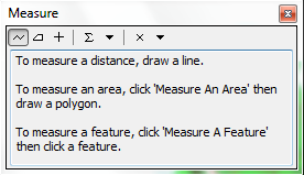
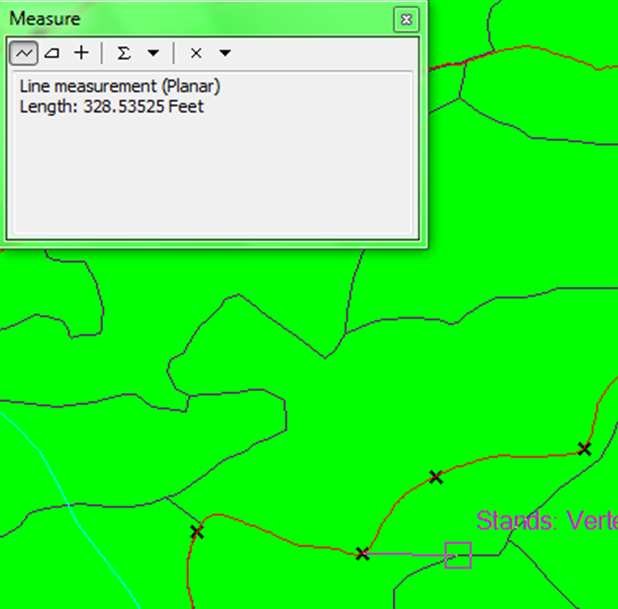
- Click the Measure tool
 . The Measure
dialog will open.
. The Measure
dialog will open.
- The pointer will change to an L-square
 ,
and when you click on a location, you will see a line between the place you
clicked and the pointer. You will also notice that the window above reports
the length of the line.
,
and when you click on a location, you will see a line between the place you
clicked and the pointer. You will also notice that the window above reports
the length of the line.
- To change the line's shape, single click again on the view. As you keep
clicking, the shape of the line will change, adding a vertex at each point
where you click. Segment means the length of current segment
of the line (if you click multiple times on the screen). And Length
means the total length for the line which you draw.
- To finish the line, double-click on the view, or hold the
<CTRL> key and single-click the mouse.
- You can also measure area of shapes by creating shapes using one of the
area measurement tools on the widow (see below)
-
click the trapezoid
shape at the top bar of this window. And like line measurement, you can click
on the screen multiple times to see how the measurement is updated by your
clicking.
Summary: You have just measured lengths and areas on a view. This is
similar to using a measuring wheel or a dot grid or planimeter on a map, but
this method is faster, easier, and potentially more accurate. One of the biggest
differences between using this method and using a planimeter or other manual
tool is that the line or polygon you have used to measure length or area is
visible; after using a map wheel or planimeter, there is no traced outline on
the paper map. Making simple measurements is one of the basic functions of a
GIS. We will work later at getting more precise areas of polygonal features
such as vegetation patches.
Get information about features
Next, we will find features within layers based on text-formatted attribute
values in the attribute tables. You can use this to find features if you know
specific text values within the attributes.
- Turn off all layers but Stands. The easiest way to do this is to
hold the <CTRL> key down and click any of the checked checkboxes,
which turns off all layers. Then click the checkbox for Stands. Also
right-click and Zoom to layer.
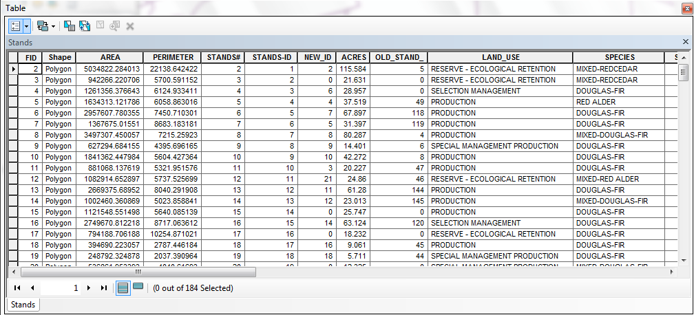
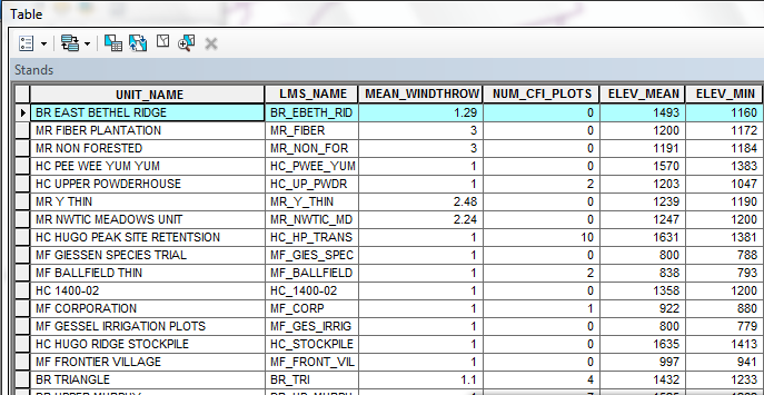
- Right-click the Stands layer name, and select Open Attribute
Table. The table contains a single record for each single stand polygon.
The records contain various pieces of data about each stand.
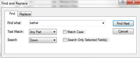
- Click Options and select Find & Replace. Search for a
stand whose name contains the word "bethel" (one of the formed Deans
of the College of Forest Resources was named James Bethel, for whom the stand
is named). Make sure to uncheck Match Case and Search Only Selected
Field(s).
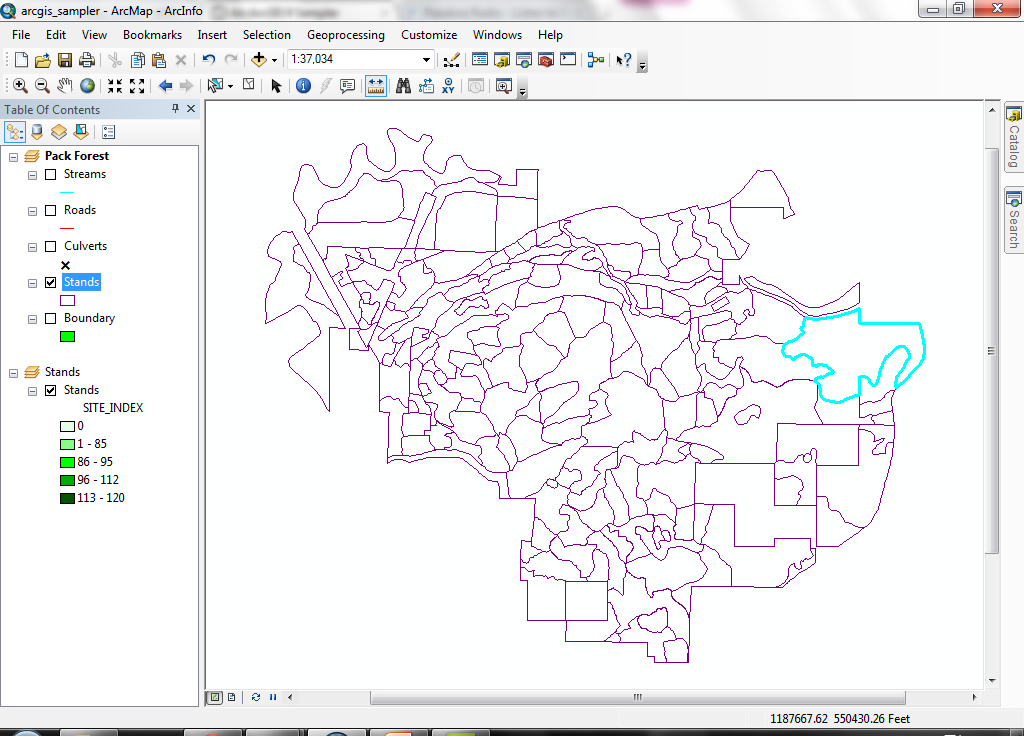
ArcGIS searches for all attributes in the layer's attribute table, and selects
any features whose text attributes contain the text you typed in. You will
see the stand selected (shaded in yellow) whose name contains the word "bethel,"
and the view will be centered on the selected feature. Searches using this
method are by default case-insensitive, so this method will match any text
string containing the letters "bethel," "Bethel," or "BETHEL."
If you want to match by case, make sure Match Case is checked. The
table will scroll to the first match, and the cell containing the text will
be outlined in bold.
- Click the leftmost column in the table (shown above with an arrowhead).
This will select the record.
Selecting the record will also select the related feature from the map.
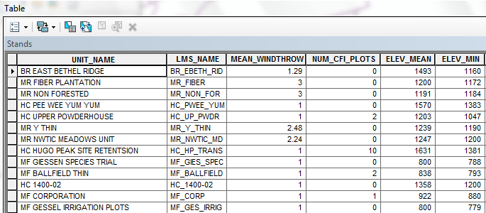
- Clicking Find Next finds the next stand matching the name search.
Use the <CTRL> key to select the second matching record. You
will see both features selected:
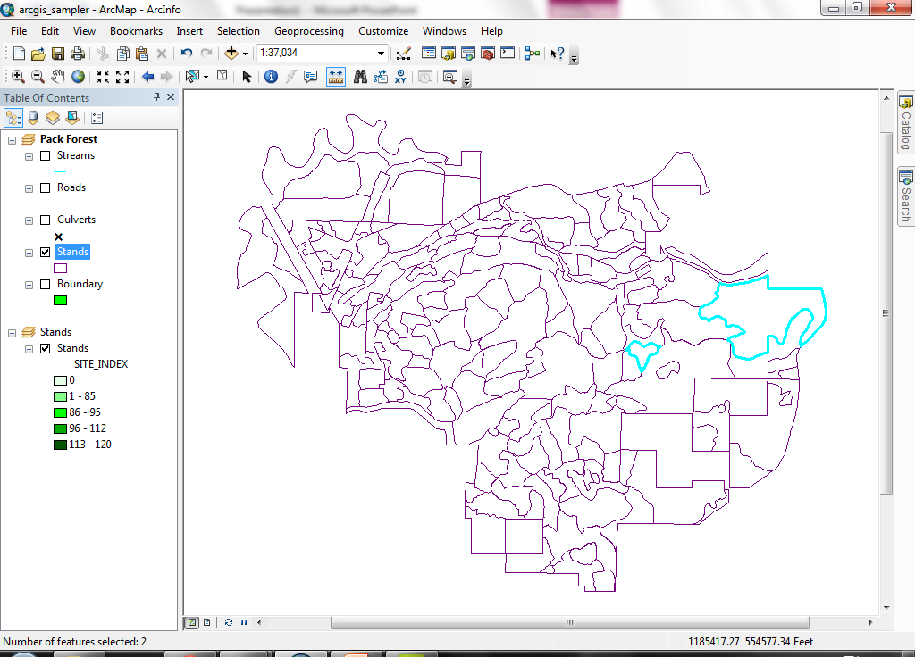
- The table shows that two records are selected.
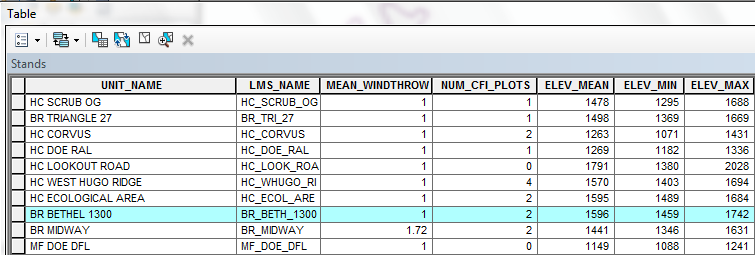
To view only those records, click the Selected button.
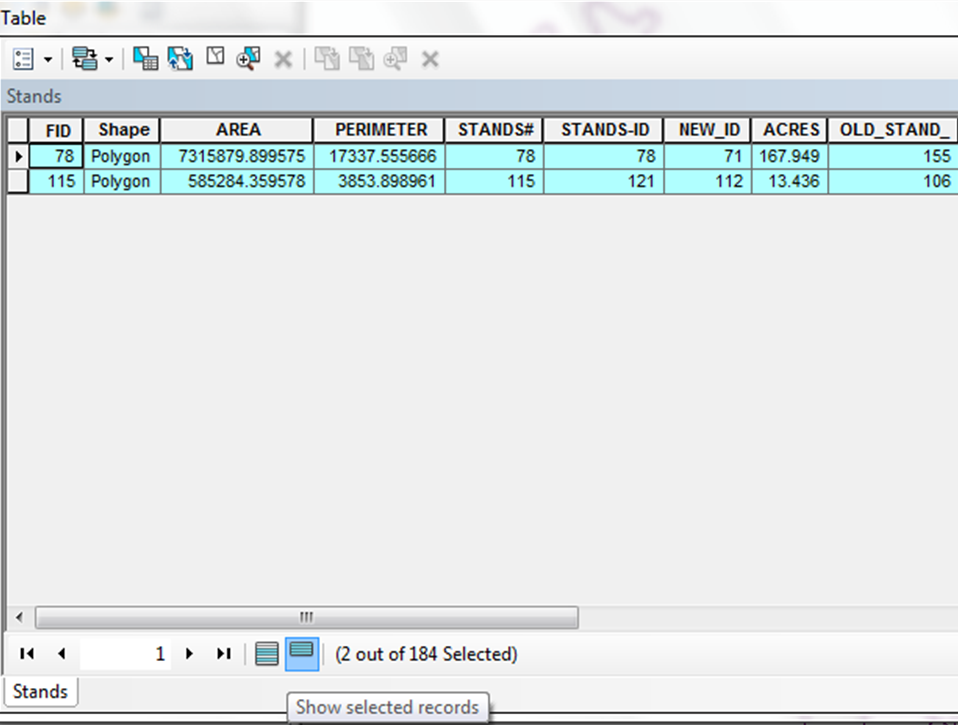
- Use the Identify tool to find out the names of these forest stands.
You will see why they matched in the text attribute search.
Continuing to click Find Next will ultimately result in no more matches.
The reason for this is that the Find functionality searches only once
through the attribute table. When it reaches the end of the table, it does
not start again at the beginning. This prevents you from continuously cycling
through a large table.
This method is good for finding features if you already know something about
the dataset's attribute values. The tool is only useful for searching for
text attributes (numeric attributes cannot be searched in this manner). Of
course, if you have no idea what text values are in the table, this method
of finding features will be of little value.
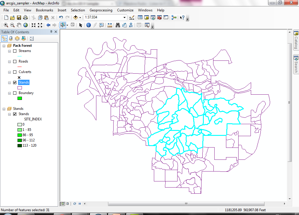
- Another way to select features is by using the Select tool
 . Click on single features or click and drag
a rectangle. Any features that are clicked or which fall partially or completely
within the rectangle will be added to the selected set. Your selection may
vary, but it should look basically like this:
. Click on single features or click and drag
a rectangle. Any features that are clicked or which fall partially or completely
within the rectangle will be added to the selected set. Your selection may
vary, but it should look basically like this:
When clicking features, the active area of the select pointer is a 3-by-3
pixel window. If you are zoomed to a very small scale, clicking on a single
feature may result in too large of a selection, and you may need to zoom in
closer.
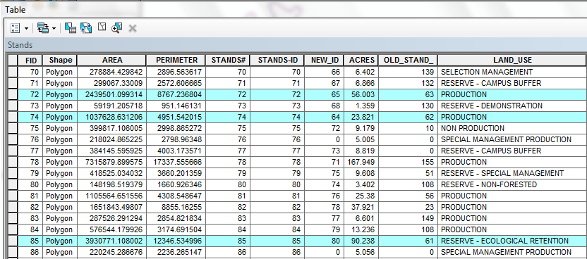
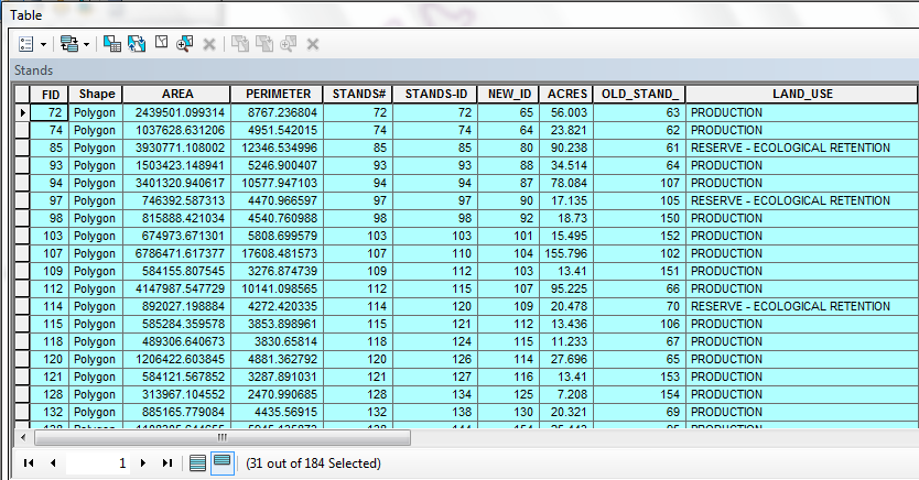
- Once you have selected a group of features, open the Stand layer's
attribute table (if you have closed it). The layer's attribute table will
open, with several records selected (the selected records, shown in cyan,
represent the selected stands in the view). You may need to scroll down the
table to see selected records.
- To view only those records, click the Selected button.
- Now sort the table according to theAge_class_2003 item. Click on the field's name in the table to make
it the active field (the field contents will be shaded in cyan), right-click,
and then select Sort Ascending.
- As you scroll, note how the table is sorted. You will see that the table is
sorted by alphabetical value, rather than numeric value (e.g., 190 < 20
in ASCII/alphabetical order). This is because the age class field is
a character field, rather than a numeric field. Be aware that the field type
will affect what type of functions can be performed on the field. We will
look at fields in more detail later in the lesson on tables.
- The section of the course on tables will delve deeper into making selections
using tabular queries. For now, unselect the selected records by clicking
the All button and then Options > Clear Selection.
Summary: You have just searched for features containing specific values,
selected features and looked at their values, opened a attribute table, and
promoted records. This is the beginning of our exploration of the relationship
between the coordinate features of a layer, and the tabular records of the layer's
table. Nearly all of what we will do in GIS will take advantage of the relationship
between layer coordinate and tabular databases.
Display and modify a table
Tables can be modified in their display properties. Fields can be hidden, renamed,
resized, and the order of records can be changed. Often, data developers give
fields cryptic names that are not easy to work with. If this is the case, you
can change the text for a field's name display.
- Right-click the Stands layer name and select Properties.
- The layer's properties will be displayed in a dialog. Click the Fields
tab. Each field is listed, with a checkbox for visibility, the Field
name, and field Alias, and a number of different properties. To hide
fields, uncheck their Visible property check box. To change the display
name of a field, enter text in the Alias box.
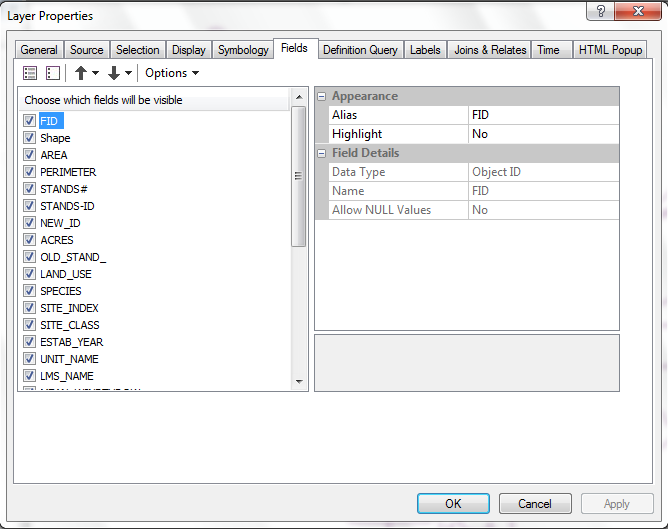
- Uncheck several of the fields.
- Scroll down to the item Age_class_2003, and enter "Current Age
Class" in the Alias box.
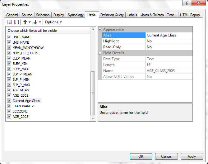
- When you OK the change, you will see the table's display change accordingly.
These changes are temporary to the ArcGIS project, and do not change the files
on the disk. This means that if you open the dataset in another project, or
even again in the same project, it will appear the same as it did before you
made these recent changes.
This can be very handy if you get a layer with a table that contains many
attribute fields, but you are interested in displaying only a few fields.
- Make the Age_2003 field active, and click the Sort Ascending button
again, and the records will be placed in the correct order.
- Close the attribute table, and zoom to the full extent of all the layers
by clicking the Zoom to Full Extent button .
Summary: You have just opened a layer's table, and altered its properties
(turned field display off, altered the field name alias) . You have also sorted
the table's records. None of these changes affect the table's file source on
the disk.
Display and modify a graph
- Right-click the Stands data frame title
 and select Activate. This will switch data frames.
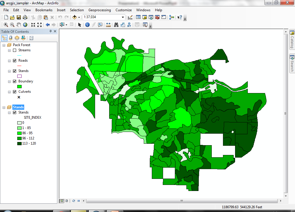
- The Stands data frame shows Pack Forest's forest stands. The stands
are classified into 5 natural-break classes based on the Site_index
field in the feature attribute table. (For those of you that do not know,
site index is an estimate of the height of a tree at 50 or 100 years for a
particular area; the larger the site index, the more productive the location.)
- Open the attribute table for the Stands layer. Note the item Site_index.
I have prepared a summary table of the layer attribute table, in which the
area per site index value is summed. This table is saved as Site Index.
You will download this summarized table in the next step.
- Download the site_index.dbf file into the main (root) directory of your removable drive. (Note:
make sure the file you downloaded has the name site_index.dbf. Web
servers and browsers can arbitrarily rename files. If the file has a different
name, rename it to the correct name. If you do not know how to view file names
and extensions, go through this
short tutorial.)
- Click Source tab in the table of contents. You can see where your
data comes from (you can find the pathname for this dataset). Switch the active data frame to Pack Forest
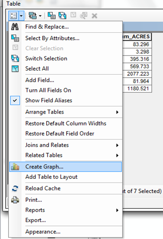
- To create the graph, open the site_index table, select Create graph from the Table Option. After this click, you will see the Create Graph Wizard.
- Fill the information as shown below.
- Choose Value field: Sum_ACRES
- Choose X label field: SITE_INDEX
- Check "Show labels (marks)"
- Choose Color: Palette Classic
- Click Next
- Change the title to Site Index Distribution
- Click Finish and you may need to resize the graph window. You can see the
area (in acres) of each site index class.
- If you want to change the format of the graph into a pie graph by right-clicking
the title bar for the graph and selecting Properties.
- Use the following settings:
- Choose Graph type: Pie
- Choose Value field: Sum_ACRES
- Choose Label field: SITE_INDEX
- Choose Color: Palette Classic
- Check Show labels (marks).
- Click OK and you can see the graph below.
Now your data show the relative proportion of area of each site class to
the entire forest.
- The problem with this graph is that the colors on the graph do not match
the colors on the map in the view. It is difficult to see the spatial arrangement
of the classes summarized in the graph. Finally, you will change the display
properties of the view to match the colors of the pie graph. Presently the
view displays site classes in a green monochrome color ramp, but we want the
colors in the view to match the graph.
- Switch the active data frame back to "Stands".
- Download the file site_index.lyr
(place it in the root of the removable drive). (Note: using the Windows
Explorer, make sure the file you downloaded has the name site_index.lyr.
Web servers and browsers can arbitrarily rename files that have been downloaded.
If the file has a different name, rename it to the correct name.)
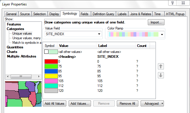
- Currently the legend displays the Site_index field in 5 classes,
using a green monochromatic color ramp. Open the properties for the Stands
layer in the table of contents. Click the Symbology tab.
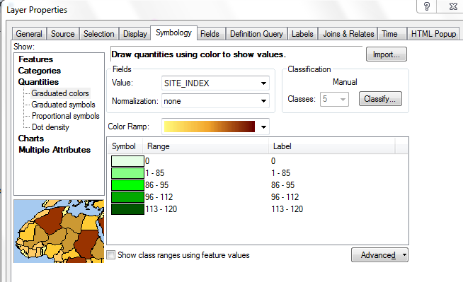
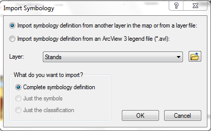
- Click the Import button. Navigate to your removable drive and
add the site_index.lyr file you just downloaded.
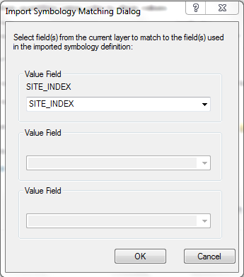
- Make sure the Value Field dropdown is set to SITE_INDEX.
Click OK.
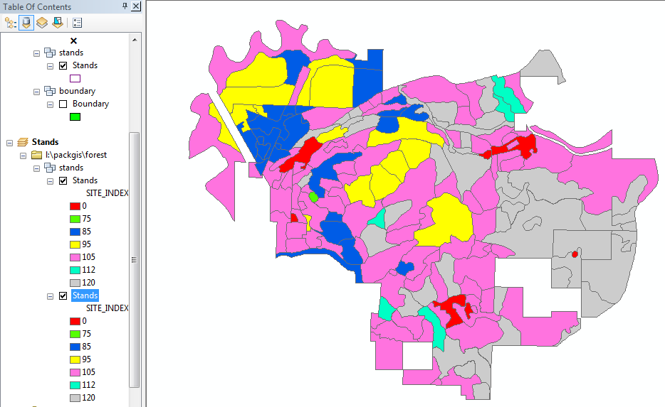
You will see that the symbology has been updated. You are loading a pre-prepared
ArcGIS legend file that will alter the colors of the display for
the Stands layer. If you create a customized legend for a layer
and you wish to use that legend over again, you can save it in one project,
then load it in another. This saves the time of re-creating the legend
from scratch.
Click OK.
- Now you can see not only the relative proportion, but also where the different
site indexes are distributed across the forest. White polygons are unclassified
or are outside the administrative boundary.
Summary: You have just looked at a graph and altered its properties.
Charts are used to make numeric data more easily understood. You have also downloaded
a ArcGIS legend file to load a predefined classification and legend for a layer.
Later, you will learn to alter the layer legends on your own.
Create a layout
In a map layout, you can place graphical elements containing views, graphs,
tables, images, and graphical primitives on a page. The layout can then be sent
to a printer or plotter, or saved as a graphics file. This step in the exercise
will create a simple map from the site index view.
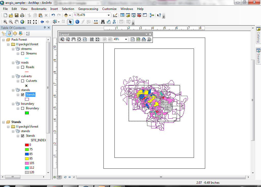
- Click the Layout View button
 at the lower left of the map display. This will change from data view to layout
view.
at the lower left of the map display. This will change from data view to layout
view.
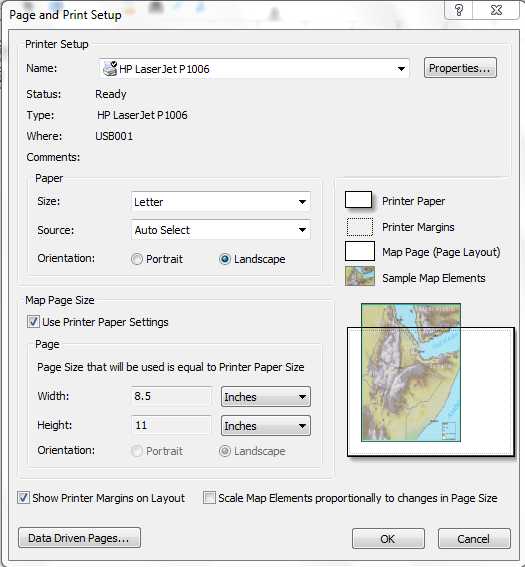
- Change from portrait to landscape orientation (File > Page and Print
Setup, select Landscape). Also make sure that Scale Map Elements
proportionally... is checked.
- There are two data frames in the map. Click and drag the the data frame
for the Pack Forest data frame off the layout. Resize and move the
other data frame to fit the page better.
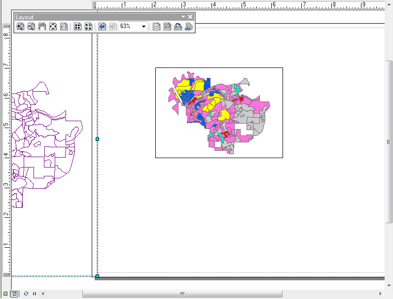
Summary: You have just created a simple map layout. As you know, one
of the main uses of GIS is to create maps. This simple layout results in a map
that is too generic for most purposes. We will spend one class session on creating
and modifying layouts later in the course.
You can use the method described for creating
PDF files to create PDF files of map compositions for distribution via e-mail
or the web. It is also possible to export layouts in a number of different graphical
file formats.
Close the project
You have just experienced a cursory view of what ArcGIS has to offer. Each
of the topics covered in this first exercise will be covered in greater detail
later in the term.
For now, close ArcMap. When asked if you want to save the document, click Yes.
Open a Windows Explorer and view the contents of the removable drive. You should
see the project you just downloaded and modified (arcgis_sampler.mxd),
the dBASE file you downloaded (site_index.dbf), and the layer file (site_index.lyr).
Get used to looking at the file system and knowing what files represent what
datasets.
REMEMBER TO TAKE YOUR CD AND REMOVABLE DRIVE
WITH YOU!!!!
Return to top
 |
|
TThe University of Washington Spatial Technology, GIS, and Remote Sensing
Page is supported by the School of Forest Resources
|
|
School of Forest Resources
|
 UW
Home
UW
Home