Chapter 16 ANOVA: Part 1 - The Ratio of Variances
Up to this point, our hypothesis tests have all followed the same logic: compare what we observed to what we would expect if the null hypothesis were true. In the \(\chi^2\) tests, we compared observed counts to expected counts under a model of no difference or independence. In Analysis of Variance (ANOVA), we follow the same idea, but instead of working with frequencies, we work with variability in sample means.
In this chapter we’ll introduce ANOVA the traditional way, which involves comparing ratios of variances and the F-distribution. Later on we’ll get into how to conduct ANOVA tests using linear regression which is a different way of looking at the same thing.
The one-factor ANOVA is a way of comparing multiple means to each other. It’s really an extension of the two-sample t-test which is for just two means.
You can find this test in the flow chart here:

In fact, you can run an ANOVA test with two means and you’ll get the exact same results. You might be wondering why we even bothered with t-tests. I guess there are two reasons. First, z and t-tests are good ways of introducing the concepts of hypothesis testing, including effect sizes and power. Second, the omnibus ANOVA F-test is non-directional: it tests whether any means differ, not whether one specific mean is larger. If you want a directional (one-tailed) test for a specific contrast, you typically use a t-test on that comparison.
16.1 Generating a Fake Data Set
We’re going to generate a random data set to work with. Creating fake data may seem like a weird (and wrong) thing to do, but it’s a very powerful way of testing out your analysis methods. I recommend to my students that they create and analyze a random data set before they even start their experiment. It’s not hard to do, and it lets you not only debug your code beforehand, but it also can reveal problems in your experimental design, and even let you estimate the power of your experiment.
For this example, suppose you think there might be a difference in final exam scores for a class that you’ve been teaching over the years. There were always the same number of students in the class, and each class had a different set of students. If there were only two years, we’d conduct a two-sample t-test for independence.
Here’s some code that will generate a fake data set of scores by drawing from a normal distribution of known mean and standard deviation. We can think of the mean and standard deviation as the population parameters.
set.seed(0)
n <- 16  # number of students per class
k <- 5   # number of classes
mu <-70  # population mean
sigma <-8  # population standard deviation

dat <- as.data.frame(matrix(nrow = n,ncol = k))
colnames(dat) <- sprintf('Year %d',seq(1,k))
for (i in 1:k) {
  dat[,i] <- round(rnorm(n,mu,sigma))
}
There’s a bit to unpack here. The command set.seed(0) sets the random number generator seed to some chosen number. Setting the seed (to any value) determines the list of randomly generated numbers to follow. If you set the seed before generating the data set you will always generate the same ‘random’ data set. You’ll get the same list of numbers as me if you set the seed to zero.
The command dat <- as.data.frame(matrix(nrow = n,ncol = k)) creates a data set of the desired size but full of NA’s. It’s a way of setting aside space to be filled in later.
The command colnames(dat) <- sprintf('Year %d',seq(1,k)) is a tricky way of generating a list of names ‘Year 1’, ‘Year 2’, etc. of length k which are used as the names of each column.
Finally, the for loop loops through k times, each time filling in the ith column with random numbers generated from a normal distribution with meanmu and standard deviation sigma. dat[,i] is a way of referring to every element of the ith column. dat[i,] will give you the elements of the ith row.
| Year 1 | Year 2 | Year 3 | Year 4 | Year 5 |
|---|---|---|---|---|
| 80 | 72 | 67 | 77 | 63 |
| 67 | 63 | 65 | 68 | 72 |
| 81 | 73 | 76 | 72 | 59 |
| 80 | 60 | 79 | 67 | 73 |
| 73 | 68 | 78 | 90 | 72 |
| 58 | 73 | 67 | 64 | 71 |
| 63 | 71 | 80 | 70 | 70 |
| 68 | 76 | 68 | 72 | 72 |
| 70 | 70 | 84 | 75 | 65 |
| 89 | 74 | 74 | 69 | 69 |
| 76 | 79 | 66 | 52 | 75 |
| 64 | 64 | 63 | 60 | 79 |
| 61 | 60 | 61 | 73 | 71 |
| 68 | 70 | 61 | 70 | 69 |
| 68 | 68 | 57 | 62 | 63 |
| 67 | 66 | 79 | 69 | 58 |
Each column was generated from a normal distribution with the same mean (\(\mu_{x}\) = 70) and standard deviation (\(\sigma_{x}\) = 8). So these differences between means are just due to random sampling. More formally, you can think of this data set as being drawn from a world where the null hypothesis is true. We write this as:
\(H_{0}: \mu_{1} = \mu_{2} = ... = \mu_{k}\)
All population means are equal.
Let’s see how different these test scores are by creating a table of summary statistics - the sample size, the mean, standard deviation and variance for each year. We’ll get fancy and use the apply function. For example sapply(dat,mean) will calculate the mean of each column of dat. We’ll also round to two decimal places to make things prettier. It’s called ‘apply’ because it applies the function to every column.
summary <- data.frame(n = sapply(dat,length),
                      mean = round(sapply(dat,mean),2),
                      sd = round(sapply(dat,sd),2),
                      var = round(sapply(dat,var),2))
Here are our results:
| n | mean | sd | var | |
|---|---|---|---|---|
| Year 1 | 16 | 70.81 | 8.39 | 70.43 |
| Year 2 | 16 | 69.19 | 5.50 | 30.30 |
| Year 3 | 16 | 70.31 | 8.23 | 67.70 |
| Year 4 | 16 | 69.38 | 8.26 | 68.25 |
| Year 5 | 16 | 68.81 | 5.75 | 33.10 |
The means differ by a few points. But how different are they?
We actually know how much they should differ, on average, thanks to the Central Limit Theorem. Since each sample is from a normal distribution with a mean of \(\mu_{x}\) = 70 and standard deviation of \(\sigma_{x}\) = 8, each mean with sample size n = 16 is drawn from a normal distribution with standard deviation:
\[ \sigma_{\bar{x}} = \frac{\sigma_{x}}{\sqrt{n}} = \frac{8}{4} = 2\]
We have 5 means. On average the standard deviation of these 5 means should be equal to 2. Let’s calculate the standard deviation of our means, which we can call \(s_{\bar{x}}\). We’ll use sapply again to get the mean of each sample, and then take the standard deviation:
## [1] 0.8319781This number 0.832 is kind of close to the expected value of \(\sigma_{\bar{x}}\) = 2.
Now, since
\[\sigma_{\bar{x}} = \frac{\sigma_{x}}{\sqrt{n}}\],
We know that
\[\sigma_{x} = \sigma_{\bar{x}}\sqrt{n}\]
It follows that since \(s_{\bar{x}}\) is an estimate of \(\sigma_{\bar{x}}\), if we multiply \(s_{\bar{x}}\) by \(\sqrt{n}\) we should have an estimate of \(\sigma_{x}\). This gives us (0.832)(4) = 3.3279.
Which is kind of close to 8.
The ‘V’ in ANOVA is for ‘Variance’, so let’s start thinking in terms of variance. The variance of the population, \(\sigma^{2}_{x}\), is \(8^{2} = 64\). Instead of comparing \(s_{\bar{x}}\sqrt{n}\) to estimate \(\sigma\), we’ll square it to get \(n \cdot s^{2}_{\bar{x}}\) and compare it to \(\sigma^{2}_{x}\). For our data set, \(n \cdot s^{2}_{\bar{x}}\) can be calculated like this:
## [1] 11.075Which is an estimate of the population variance \(\sigma^{2}_{x}\) = 64.
This gives us a hint for how we can test our null hypothesis. When \(H_{0}\) is true, each time we calculate \(n \cdot s^{2}_{\bar{x}}\) we should get a number that is close to the population standard variance \(\sigma^{2}_{x}\).
Now, suppose what happens when \(H_{0}\) is false, and the population means are not all the same. This will make the variance the means larger, on average, so we should, on average, get values of \(n \cdot s^{2}_{\bar{x}}\) that are larger than 64.
From our fake data set, we could run a hypothesis test comparing our observed value of \(n \cdot s^{2}_{\bar{x}}\) = 11.075 to 64 and reject \(H_{0}\) if it gets big enough.
But we don’t normally know the population variance \(\sigma^{2}_{x}\). What can we use instead?
We have 5 samples of size 16 drawn from a normal distribution with variance \(\sigma^{2}_{x}\) = 64. Look back at the table, are the variance of each of these samples around 64? They should be.
To combine these 5 variances into a single number we’ll take the mean.
Using R, we first calculate the variance of each sample (using `var andsapply(dat,var)), then take the mean:
## [1] 53.95333This number is fairly close to \(\sigma^{2}_{x}\) = 64. Notice, however, that this number shouldn’t change, on average, with differences in the mean. This makes this number an estimate of the population standard deviation even if \(H_{0}\) is false.
One way to think about ANOVA is that it’s about comparing two numbers - the variance of the means (times n) to the mean of the variances.
The statistic we compute is the ratio of these two numbers. For our example, this ratio can be computed in one step:
## [1] 0.20527This ratio of variances is called an F statistic, which is why I’ve called it F_obs for ‘F observed’.
If \(H_{0}\) is true, then F_obs should around 1 on average since both are estimates of the same number, the population variance \(\sigma^{2}\).
How unusual is our ratio of 0.21?
We can answer this by generating a huge set of fake data sets and calculate the F-statistic for each set.
nReps <- 10000  # number of fake data sets

datj <- as.data.frame(matrix(nrow = n,ncol = k))
colnames(datj) <- sprintf('Year %d',seq(1,k))

Fs <- numeric(nReps)  # allocate a vector of zeros to be filled in

for (j in 1:nReps) {
  for (i in 1:k) {
    datj[,i] <- round(rnorm(n,mu,sigma))
  }
  # Calculate the F statistic for this data set and save it in Fs[j]
  Fs[j] <- n*var(sapply(datj,mean))/mean(sapply(datj,var))
}
The code above loops through 10000 times, each generating a fake data set like before. For each fake data set, an F-statistic is calculated and is saved in the vector ‘Fs’.
Let’s look at a histogram of our 10000 F statistics. I’m hiding the code so we can keep things moving.
It’s a strange looking distribution. First you’ll notice that all values are positive - that’s because we’re working with variances which are always positive. Second, you’ll notice that it is strongly positively skewed. Third, the mean of the distribution is around 1. This should make sense, since this is the expected ratio if \(H_{0}\) is true.
This F-distribution has a known ‘parameterized’ shape, like the z-distribution and t-distribution. Like t, it’s a family of distributions, but the F-distribution requires two separate degrees of freedom, one for the numerator and one for the denominator. Formally, the F distribution is the ratio of two \(\chi^2\) distributions. For more on this, check out this section on the chapter about how all distributions in this book are based on the normal distribution.
The df for the numerator is k-1, where k is the number of means: 5 - 1 = 4 for our example. For the denominator, which is the mean of the variances, each sample contributes n-1 degrees of freedom, so the total df for the denominator is \(k(n-1)\) = \(5(16-1) = 75\). This is the same as nk - k, which can be written as N-k where N is the total number of scores in the experiment (nk).
You can find areas under the F distribution using R’s pf function, which functions like the pnorm and the pt functions for normal and t-distributions. Here’s the histogram of our generated F-statistics along with the known F-distribution with 4 and 75 degrees of freedom.
You can see that our randomly sampled F-statistics nicely fit the known F-distribution. The F-statistic for our first randomly generated data set was 0.21. Where does this sit compared to the F-distribution?
R’s pf function finds the area below a given value of F. So the area above our observed statistic is:
## [1] 0.934734This isn’t a very unusual draw from the distribution. If we choose \(\alpha\) = 0.05, we wouldn’t be suspicious that the null hypothesis is not true.
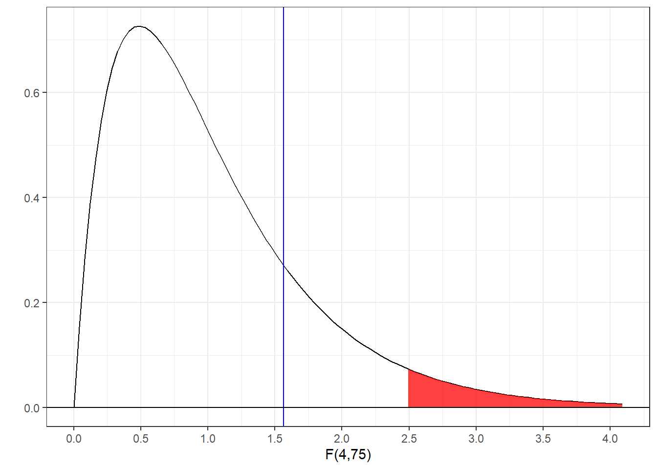
R’s qf function is like qnorm and qt - it provides the value of F for the upper percentile. If we let \(\alpha\) = 0.05, the F-statistic that defines the top 5% is:
## [1] 2.493696We need a F-statistic of 2.49 or more to reject \(H_{0}\).
Here’s the known F-distribution with the top 5% shaded in red, and our observed value of F as a vertical line:

For this random data set, our observed value of F does not fall in the critical region, so we’d fail to reject \(H_{0}\) and we could not conclude that our samples were drawn from populations with different means.
If we were to change the random seed, we’d get a different F-statistic. One out of 20 times we’d expect to land in the rejection region by chance. We know that this would be a Type I error because we know that \(H_{0}\) is true.
In fact, we did generate 10000 data sets and F-statistics. We can count the proportion of our randomly generated F-statistics that fall above the critical value:
## [1] 0.0456456 out of the 10000 F-statistics are greater than 2.49. This is very close to proportion of \(\alpha\) = 0.05.
16.2 Simulating data when \(H_{0}\) is false
In this last part we’ll generate a whole new set of fake data, but this time we’ll make \(H_{0}\) be false. This code is much like the code above:
# set mus and sigmas to be vectors for population means and sd's
mus <- rep(70,k)
sigmas <- rep(8,k)

# reset the first mean to be 75
mus[1] <- 75

datj <- as.data.frame(matrix(nrow = n,ncol = k))
colnames(datj) <- sprintf('Year %d',seq(1,k))

Fs <- numeric(nReps)  # allocate a vector of zeros to be filled in

for (j in 1:nReps) {
  for (i in 1:k) {
    # use each sample's mean and sd to generate the sample
    datj[,i] <- round(rnorm(n,mus[i],sigmas[i]))
  }
  # Calculate the F statistic for this data set and save it in Fs[j]
  Fs[j] <- n*var(sapply(datj,mean))/mean(sapply(datj,var))
}
The only difference is that we now have a vector of numbers for the population mean and standard deviations, called mus and sigmas. We set all of the sigmas to be the same, but we changed the first mean from 70 to 75.
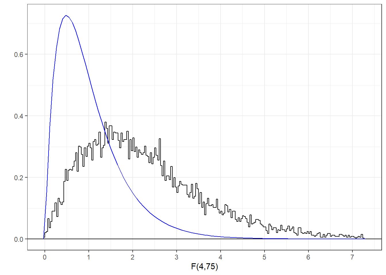
Here’s a histogram of our new set of randomly generated F-statistics along with the known F-distribution:

This no longer a good fit. We’re generating way too many large F-statistics. This is because by changing that first mean, we’ve increased the numerator of F, the variance of the mean across our samples, without increasing denominator, the average mean of the variances.
Now if we calculate the proportion of F-statistics that fall above our critical value:
## [1] 0.371We now reject \(H_{0}\) much more often than 5% of the time.
Since \(H_{0}\) is false, rejecting \(H_{0}\) is the correct decision. Do you remember what we call the proportion of times that we correctly reject \(H_{0}\)?
It’s power.
We just used a simulation to estimate the power of our ANOVA when we made \(H_{0}\) false in a very specific way.
I hope you appreciate the ‘power’ of this sort of simulation. You don’t need to know any math. All you need to do is generate fake data sets with some chosen set of population parameters and count the number of times that you reject \(H_{0}\). This sort of procedure can be used for any sort of hypothesis test. It’s also a sanity check for \(H_{0}\), since if you set your population parameters so that \(H_{0}\) is true (like we first did), your simulations should lead to rejections around a proportion of \(\alpha\).
16.3 F Widget
You can run simulations yourself with the following widget. You can choose the number of levels (k) and the sample size for each level (n), the means and standard deviations for each level and \(\alpha\). Click the ‘STEP’ button and you’ll generate a single simulated data set, along with where the F-static lands. Click ‘GO’ and it’ll start simulating multiple simulated data sets, and you’ll see the histogram of F statics build. If the means are all the same (\(H_0\) is true), then the histogram of F-statistics should converge toward the theoretical F-distribution, and you should be rejecting \(H_0\) \(\alpha\) proportion of the time.
Now, if you make the means different, then you should start rejecting \(H_0\) with a proportion more than \(\alpha\). That’s the power! If you click the ‘show noncentral F’ toggle box, you’ll see the smooth F-distribution shift to something closer to building histogram. This is the theoretical distribution of F-statistics for this particular set of means and standard deviations.
If this is broken, or you’re looking at a pdf or printout you can run the demo at https://gboynton.github.io/F/.