Chapter 17 Apriori and Post-Hoc Comparisons
ANOVA tells us that at least one mean differs, but it does not tell us which means differ. To answer that question, we use comparisons. This chapter is about how to test hypotheses that are more specific than the original omnibus ANOVA. Examples include comparing just two of the means, or comparing one mean (e.g. a control condition) to each of the other means.
The main issue here is familywise error, FWER discussed in the last chapter, which is that the probability of making one or more Type I errors increases with the number of hypothesis tests you make.
For example, if you run 10 independent hypothesis tests on your results, each with an alpha value of 0.05, the probability of getting at least one false positive would be:
\[1-(1-0.05)^{10} = 0.401\]
This number, 0.4013 is clearly unacceptably high. The equation above applies only to independent hypothesis tests. In most of the ANOVA post-hoc settings, the tests are typically correlated, so the exact FWER differs, but the idea is the same: FWER increases with the number of hypothesis tests.
The goal of correcting for FWER is to adjust the tests to make it harder to reject \(H_0\). Specifically, we want the the probability of making 1 or more type I errors to be less than \(\alpha\).
Specific hypothesis tests on ANOVA data fall into two categories, ‘A Priori’ and ‘post-hoc’.
A Priori tests are hypothesis tests that you planned on running before you started your experiment. Often they are written down and preregistered. Since there are many possible tests we could make, setting aside a list of just a few specific A Priori tests lets us correct for a relatively low familywise error rate.
Post-hoc tests are hypothesis tests that you came up with after looking at the data. For example, you might want to go back and see if there is a significant difference between the highest and lowest means. Under the null hypothesis, the probability of rejecting a test on the most extreme difference between means will be much greater than \(\alpha\). Or, perhaps we want to go crazy and compare all possible pairs of means. Since there are many tests that you could have run, even if you only care about a few, you need to correct for a larger FWER than if you just had a few A priori tests in mind.
17.1 One-Factor ANOVA Example:
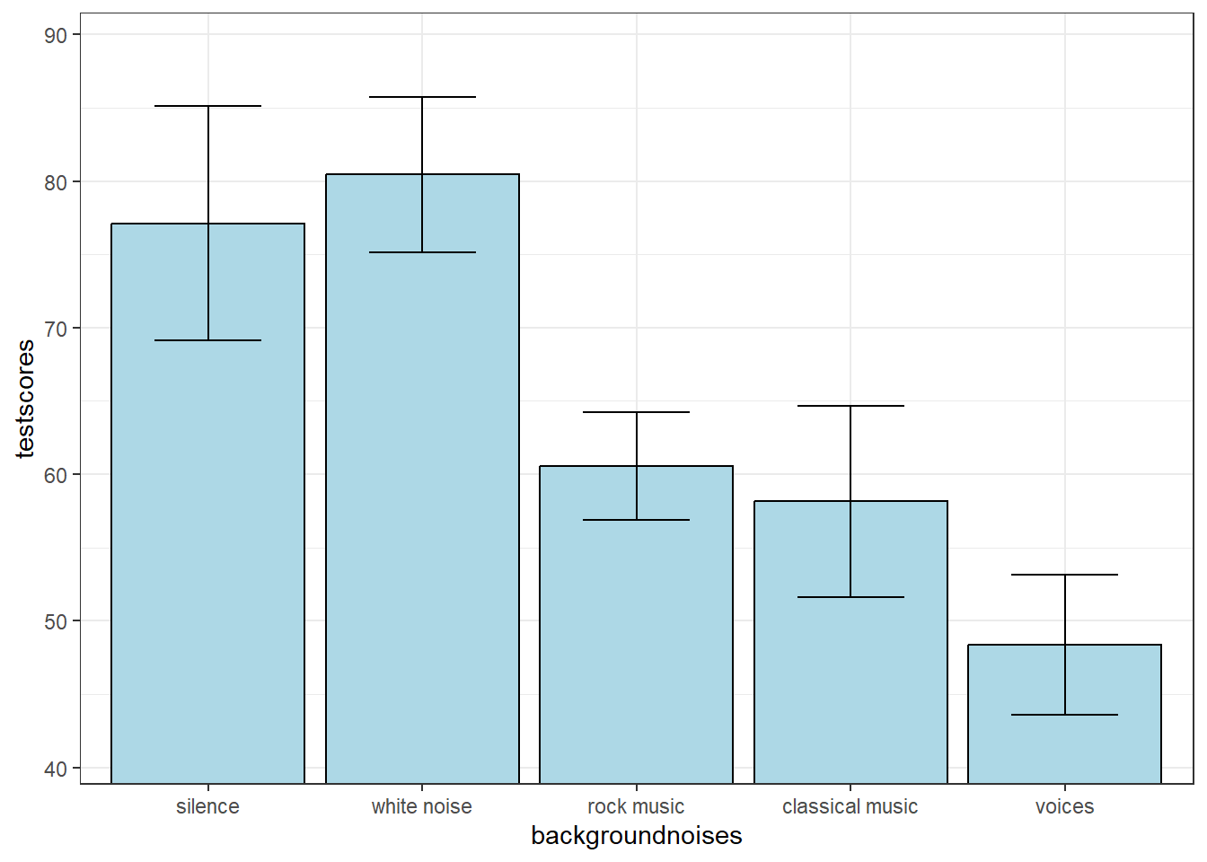
We’ll go through A Priori and post-hoc tests with an example. Suppose you want to study the effect of background noise on test score. You randomly select 10 subjects for each of 5 conditions and have them take a standardized reading comprehension test with the following background noise: silence, white noise, rock music, classical music, and voices.
Throughout this chapter we’ll be referencing this same set of data. You can access it yourself at:
http://courses.washington.edu/psy524a/datasets/AprioriPostHocExample.csv
Your experiment generates the following statistics:
| mean | n | sd | sem | |
|---|---|---|---|---|
| silence | 77.11 | 10 | 25.26436 | 7.989291 |
| white noise | 80.45 | 10 | 16.70617 | 5.282955 |
| rock music | 60.56 | 10 | 11.63856 | 3.680435 |
| classical music | 58.15 | 10 | 20.61112 | 6.517809 |
| voices | 48.37 | 10 | 15.04113 | 4.756424 |
The result of the ANOVA is:
| df | SS | MS | F | p | |
|---|---|---|---|---|---|
| Between | 4 | 7285.217 | 1821.3042 | 5.3445 | p = 0.0013 |
| Within | 45 | 15335.044 | 340.7788 | ||
| Total | 49 | 22620.261 |
Here’s a plot of the means with error bars as the standard error of the mean:
17.2 A Priori Comparisons
An A Priori test is a hypothesis test that you had planned to make before you conducted the experiment. They’re sometimes called planned comparisons.
17.2.1 t-test for Two Means
The simplest A Priori test is a comparison between two specific means. In our example, suppose that before we ran the experiment we had the prior hypothesis that there is a difference in mean test score between the silence and the voices conditions. This leads to comparing the means \(\overline{X}_{1} = 77.11\) and \(\overline{X}_{5} = 48.37\)
You’d think that we would simply conduct an independent measures two-tailed t-test using these two group means and variances, while ignoring all of the other conditions (and sometimes this is what people do). But since we have \(MS_{within}\), and if we assume homogeneity of variance, we can use this value in the denominator of the t-test since it’s a better estimate of the population variance than the pooled variance from just two groups.
The regular old t-statistic was (since we have equal sample size, n):
\[t=\frac{\overline{X}_{1}-\overline{X}_{5}}{\sqrt{\frac{s_{1}^2+s_{5}^2}{n}}} = \frac{77.11 - 48.37}{\sqrt{\frac{25.3^2 + 15^2}{10}}} = 3.091 \]
With \(df = (n-1)+(n-1) = 2n-2 = 18\).
However, we have mean-squared error within (\(MS_w\)) from the ANOVA, which is a better estimate of our population variance than \(s_{1}^2\) and \(s_{5}^2\). So we’ll use it instead of the pooled variance:
\[t= \frac{\overline{X}_{1}-\overline{X}_{5}}{\sqrt{\frac{2MS_{w}}{n}}}\]
The degrees of freedom is now N-k, since this is the df for \(SS_{within}\).
For our example:
\[t= \frac{77.11 - 48.37}{\sqrt{\frac{(2)340.8}{10}}} = 3.4813\]
With df =N-k = 50 - 5 = 45, the p-value of t is 0.0011.
Since we planned on making this comparison ahead of time, and this is our only A Priori comparison, we can use this test to reject \(H_{0}\) and say that there is a significant difference in the mean test score between the silence and the voices conditions.
As an exercise, make a planned comparison t-test between the rock music and classical music conditions. You should get a t-value of 0.2919 and a p-value of 0.7717.
17.2.2 ‘Contrast’ for two means
Another way of thinking about the comparison we just made between the means from the silence and the voices conditions is to consider the numerator of our t-test as a ‘linear combination’ of means. A linear combination is simply a sum of weighted values. If we call \(a_i\) the weight for group \(i\), then for this comparison, we assign a weight of \(a_{1} = 1\) for the silence condition and a weight of \(a_{5} = -1\) for the voices condition. All other means get zero weights. We use a lower case ‘psi’ (\(\psi\)) to indicate this weighted sum of means:
\[\psi = \sum{a_i\overline{X}_i}\]
For this example is simply difference between the two means:
\[\psi = (1)(77.11) + (-1)(48.37) = 28.7400\]
The t-statistic for any contrast is:
\[ t = \frac{\psi}{\sqrt{MS_w\sum{{(a_i^2/n_i)}}}} \]
Where \(a_i\) is the weight for for group \(i\) and \(n_i\) is the sample size for group \(i\). For equal sample sizes, like this example, the t-statistic simplifies to:
\[ t = \frac{\psi}{\sqrt{MS_w(\sum{{a_i^2})/n}}} \]
Which for our example, t is exactly as we calculated above:
\[t = \frac{28.74}{\sqrt{340.78(1^2+(-1)^2)/10}} = 3.4813\] Note that our contrast weights, 1 and -1, can vary by a scale factor. If we used, for example, \(\frac{1}{2}\) and \(-\frac{1}{2}\) we’d get the same t statistic and p-value. But the contrasts do have to add up to zero in order to test the null hypothesis that the population means are the same.
Sometimes you’ll see contrasts computed in terms of the F statistic instead of t. This is equivalent because, as we’ve discussed earlier, \(F = t^2\).
17.2.3 Contrast for groups of means
Contrasts also allow us to compare groups of means with other groups of means. In our example, suppose we have the prior hypothesis that music in general has a different effect on test scores than white noise. That is, we want to compare the average of the two music conditions (rock and classical) with the white noise condition.
Our weights will be 1 for the white noise condition, and -.5 for the rock and -.5 for the classical conditions, and zero for the remaining conditions. The corresponding linear combination of means is:
\[\psi = (1)(80.45) + (-0.5)(60.56) + (-0.5)(58.15) = 21.0950\]
You should convince yourself that this value, \(\psi\), is the difference between the white noise condition and the average of the two music conditions. It should have an expected value of zero for the null hypothesis because the weights add up to zero.
The t-statistic for this contrast is:
\[t = \frac{21.095}{\sqrt{340.78\frac{(1)^2 +(-0.5)^2+(-0.5)^2}{10}}} = 2.95\]
The degrees of freedom for all contrasts is equal to the degrees of freedom for \(MS_w\), which is 45. The p-value for this contrast is 0.005
17.2.3.1 Orthogonal contrasts and independence
We have now made two contrasts. These two contrasts are independent simply because they don’t share any groups in common. They could have come from completely different experiments.
Contrasts can be independent even if they share groups. Formally, two contrasts are independent if the sum of the products of their weights (the ‘dot product’) add up to zero. When this happens, the two contrasts are called orthogonal. In our example:
c1 = [1, 0, 0, 0, -1]
and our new contrast is
c2 = [0, 1, -1/2, -1/2, 0]
The sum of their products is 0:
(1)(0) + (0)(1) + (0)(-.5) + (0)(-.5) + (-1)(0) = 0
Another contrast that is orthogonal to the second one is:
c3 = [0, 0, 1, -1, 0]
This is because (0)(0) + (1)(0) + (-.5)(1) + (.5)(1) + (0)(0) = 0
What does this contrast test? It compares the test scores for the rock and classical music conditions. Notice that this contrast is also orthogonal to c1, the first contrast.
It turns out that there are exactly as many mutually orthogonal contrasts as there are degrees of freedom for the numerator of the omnibus (k-1). So there should be 4 orthogonal contrasts for our example (though this is not a unique set of 4 orthogonal contrasts). This leaves one more contrast. Can you think of it?
The answer is:
c4 = [1/2 -1/3 -1/3 -1/3 1/2]
Show that c4 is orthogonal to the other three. What is it comparing? It’s the mean of the silence and voices conditions compared to the mean of the other three conditions (white noise, rock and classical). This doesn’t make much sence, so we probably wouldn’t have had an A Priori hypothesis about this particular contrast.
Notice that since each contrast has one degree of freedom, the sum of degrees freedom across all possible contrasts is equal to the degrees of freedom of the omnibus ANOVA. Likewise, it turns out that the sums of the \(SS_{contrast}\) across all orthogonal contrasts adds up to the \(SS_{bet}\).
If two contrasts are orthogonal, then the two tests are ‘independent’. If two tests are independent, then the probability of rejecting one test does not depend of the probability of rejecting the other. An example of two contrasts that are not independent is comparing silence to white noise for the first contrast, and silence to rock music for the second contrast. You should see that if we happen to sample an extreme mean for the silence, then there will a high probability that both of the contrasts will be statistically significant. Even though both have a Type I error rate of \(\alpha\), there is will be a positive correlation between the probability of rejecting the two tests.
Testing orthogonal contrasts on the same data set is just like running completely separate experiments. Since orthogonal contrasts are independent, we can easily calculate the familywise error rate:
\[FWER = 1-(1-\alpha)^{n}\]
where \(n\) is the number of orthogonal contrasts.
If a set of tests are not independent, the familywise error rate still increases with the number of tests, but in more complicated ways that will be dealt with in the post-hoc comparison section below.
17.3 Contrasts with R
R has a very convenient package emmeans that has functions for conducting all of the Apriori and post-hoc analyses in this chapter.
Let’s load in the data set that we’ve been working with and compute the ANOVA. Although it’s a bit lengthy, we’ve covered this in the chapter ANOVA Part 2: Partitioning Sums of Squares:
# choose your alpha
alpha <- .05
# load in the data
mydata<-read.csv("http://www.courses.washington.edu/psy524a/datasets/AprioriPostHocExample.csv")
# reorder the levels of 'backgroundnoises'
mydata$backgroundnoises <- factor(
  mydata$backgroundnoises,
  levels = c("silence",
             "white noise",
             "rock music",
             "classical music",
             "voices"))
# run the ANOVA, saving the output of 'lm'
lm.out <- lm(testscores ~ backgroundnoises,data=mydata)
anova.out <- anova(lm.out)
To define our contrasts, we create a list of vectors, each containing the weights for the 5 levels.
contrasts <- list(
  c1 = c(1, 0, 0, 0, -1),                # silence vs voices
  c2 = c(0, 1, -0.5, -0.5, 0),           # white vs avg(music)
  c3 = c(0, 0, 1, -1, 0),                # rock vs classical
  c4 = c(0.5, -1/3, -1/3, -1/3, 0.5)     # silence+voices vs others
)
We then calculate the ‘marginal means’, which are simply the group means using the emmeans function. Note, the result is a table that is a lot like the output of summarySE - it includes the mean for each group and standard errors. However, the standard error is based on the \(MS_{w}\) from the omnibus ANOVA, not the standard deviations for each group. That’s why the ‘SE’ values in the table are all the same. As discussed earlier, all contrasts use this common value of \(MS_{w}\).
##  backgroundnoises emmean   SE df lower.CL upper.CL
##  silence            77.1 5.84 45     65.4     88.9
##  white noise        80.5 5.84 45     68.7     92.2
##  rock music         60.6 5.84 45     48.8     72.3
##  classical music    58.1 5.84 45     46.4     69.9
##  voices             48.4 5.84 45     36.6     60.1
##
## Confidence level used: 0.95
Contrasts are run using the contrast function on the output of emmeans:
##  contrast estimate   SE df t.ratio p.value
##  c1          28.74 8.26 45   3.481  0.0011
##  c2          21.09 7.15 45   2.951  0.0050
##  c3           2.41 8.26 45   0.292  0.7717
##  c4          -3.65 5.33 45  -0.684  0.4973
The ‘estimate’ is the value of \(\psi\) and ‘SE’ is the denominator of the t-test. You should recognize the \(\psi\), t, and p-values for the first two contrasts.
To access these values, you need to pass the output of contrast into summary. For example, to report the results of the first contrast:
contrast.result <- summary(contrast(emm,method = contrasts))
sprintf('t(%d) = %0.2f, p = %0.4f',  contrast.result$df[1],  contrast.result$t.ratio[1],contrast.result$p.value[1])
## [1] "t(45) = 3.48, p = 0.0011"17.3.1 Breaking down \(SS_{between}\) across contrasts
For an ANOVA with \(k\) groups there will be \(k-1\) independent contrasts. These contrasts are not unique - there can be multiple sets of \(k-1\) orthogonal contrasts. But for any set, it turns out that each of the \(k-1\) orthogonal contrasts accounts for its own portion of the variability across means, \(SS_{between}\).
To see this, we need to think of contrasts in terms of F-tests instead of t-tests. This can be done because for each contrast, the equivalent F-test would have an F value of \(F = t^2\). Also, since
\[t^2 = F = \frac{MS_{contrast}}{MS_{within}}\] since \(df_{contrast}\) = 1, \(MS_{contrast} = SS_{contrast}\), so
\[SS_{contrast}= t^2MS_{within}\] For our first contrast, \(t = 3.4813\), so, borrowing \(SS_{within}\) from the omnibus ANOVA,
If you do this for all four contrasts you’ll se that \(SS_{between}\) is the sum the \(k-1\) \(SS_{contrast}\) values:
\[4129.94+2966.66+29.0405+159.578 = 7285.22 = SS_{between}\]
The intuition behind this is that the 4 contrasts are breaking down the total amount of variability between the means (\(SS_{between}\)) into separate independent components, each producing their own hypothesis test.
17.4 Controlling for familywise error rates
The most common way to control for familywise error is to simply lower the alpha value when making multiple independent comparisons. This comes at the expense of lowering the power for each individual test because, remember, decreasing alpha decreases power.
There is a variety and growing number of correction techniques for independent tests. We’ll cover just a few here.
17.4.1 Bonferroni correction
Bonferroni correction is the easiest, oldest, and most common way to correct for FWER. All you do is reduce alpha by dividing it by the number of comparisons. For example, if you want to make 4 comparisons and want the FWER to be below 0.05, you simply test each comparison with an alpha value of 0.05/4 = 0.0125.
Our contrasts produced p-values of 0.0011, 0.005, 0.7717, and 0.4973. If we were to make all four A Priori comparisons, we’d need to adjust alpha to be 0.05/4 = 0.0125.
Using a Bonferroni correction we reject the null hypothesis for contrasts 1 and 2 but not for contrasts 3 and 4.
Equivalently, instead of dividing \(\alpha\), we can ‘adjust’ our p-values by multiplying them by 4 and compare them to 0.05. These ‘adjusted p-values’ for the Bonferroni correction can be calculated with the emmeans package by adding an ‘adjust’ argument to the contrast function:
##  contrast estimate   SE df t.ratio p.value
##  c1          28.74 8.26 45   3.481  0.0045
##  c2          21.09 7.15 45   2.951  0.0201
##  c3           2.41 8.26 45   0.292  1.0000
##  c4          -3.65 5.33 45  -0.684  1.0000
##
## P value adjustment: bonferroni method for 4 tests
Adjusted p-values are becoming the common way to report corrections for familywise error. They’re easy to interpret since they can be simply compared to \(\alpha\). Since adjusted p-values are the original p-values multiplied by the number of tests, then it’s possible for adjusted p-values to be greater than 1, which doesn’t make sense for probabilities. For those cases, adjusted p-values are set to a ceiling of 1.
17.4.2 Šidák correction
Some software packages correct for familywise error using something called the Šidák correction. The result is almost exactly the same as the Bonferroni correction, but it’s worth mentioning here so you know what it means when you see a button for it in software packages like SPSS.
Remember, the familywise error rate is the probability of making one or more false positives. The Bonferroni correction is essentially assuming that the familywise error rate grows in proportion to the number of comparisons so we scale alpha down accordingly. But we know that the family wise error rate is \(1-(1-\alpha)^m\), where m is the number of comparisons.
For example, for a Bonferroni correction with \(\alpha\) = .05 and 4 comparisons, we need to reduce the alpha value for each comparison to 0.05/4 = 0.0125. The familywise error rate is now
\[1-(1-0.0125)^4 = 0.049\]
It’s close to 0.05 but it’s just a little lower. To bring the FWER up to exactly 0.05 we need to use:
\[\alpha' = 1-(1-\alpha)^{1/m}\]
With 4 comparisons and \(\alpha\) = 0.05, the adj alpha is:
\[\alpha' = 1-(1-0.05)^{1/4} = 0.01274\]
So instead of using an alpha of 0.0125 you’d use 0.01274. The difference between the Šidák correction and the Bonferroni correction is minimal but technically the Šidák correction sets the probability of getting one or more one false alarms to exactly alpha for independent tests.
Again, the emmeans package can handle the Šidák correction by adjusting the p-values:
##  contrast estimate   SE df t.ratio p.value
##  c1          28.74 8.26 45   3.481  0.0045
##  c2          21.09 7.15 45   2.951  0.0199
##  c3           2.41 8.26 45   0.292  0.9973
##  c4          -3.65 5.33 45  -0.684  0.9361
##
## P value adjustment: sidak method for 4 tests
Notice that the adjusted p-values are just a little lower than for the Bonferroni correction.
17.4.3 Holm-Bonferroni Multistage Procedure
The Holm-Bonferroni procedure is a more forgiving way to correct for familywise error, and has been used more recently, especially for large number of comparisons. The procedure is best described by example. First, we rank-order our p-values from our multiple comparisons in from lowest to highest. From our four contrasts: 0.0011, 0.005, 0.4973, and 0.7717 for contrast numbers 1, 2, 4, and 3 respectively.
We start with the lowest p-value and compare it to the alpha that we’d use for the Bonferroni correction (\(\frac{0.05}{4} = 0.0125\)).
If our lowest p-value is less than this adjusted alpha, then we reject the hypothesis for this contrast. If we fail to reject then we stop. For our example, p = 0.0011 is less than 0.0125, so we reject the corresponding contrast (number 1) and move on.
We then compare or next lowest p-value to a new adjusted alpha. This time we divide alpha by 4-1=3 to get \(\frac{0.05}{3} = 0.0167\), a less conservative value. If we reject this contrast, the we move on to the next p-value and the next adjusted alpha \(\frac{0.05}{2}=0.025\).
This continues until we fail to reject a comparison, and then we stop.
The idea is that if you manage to reject with the lowest p-value using the full Bonferroni correction for m tests (\(\frac{\alpha}{m}\)), then you can move on to the next p-value and correct only for the remaining m-1 tests (\(\frac{\alpha}{m-1}\)), and so on.
Here’s how to run the Holm-Bonferroni procedure with the contrast function in emmeans:
##  contrast estimate   SE df t.ratio p.value
##  c1          28.74 8.26 45   3.481  0.0045
##  c2          21.09 7.15 45   2.951  0.0151
##  c3           2.41 8.26 45   0.292  0.9946
##  c4          -3.65 5.33 45  -0.684  0.9946
##
## P value adjustment: holm method for 4 tests
What you get are the adjusted p-values - so that for our example, the lowest p-value gets multiplied by 4, the second lowest is multiplied by 3 and so on. The nice thing about thinking in terms of adjusted p-values (instead of adjusting \(\alpha\)) is that the stop rule is implicit - once the first test is rejected with an adjusted p-value greater than \(\alpha\), all of the other tests will also be rejected.
17.5 Post Hoc Comparisons
Now let’s get exploratory and make some comparisons that we didn’t plan on making in the first place. These are called post hoc comparisons. For A Priori comparisons, we only needed to adjust for the FWER associated with the number of planned comparisons. For post hoc comparisons, we need to adjust to not just the comparisons we feel like making, but for all possible comparisons of that type that we could have made (e.g all possible pairwise comparisons or all possible contrasts). The more possible tests that you correct for, the greater penalty for FWER, and therefore the lower the power. The following post hoc tests test for increasing numbers of possible tests, and therefore decreasing levels of power.
17.6 Dunnett’s Test for comparing one mean to all others
This is a post-hoc test designed specifically for comparing all means to a single control condition. For our example, it makes sense to compare all of our conditions to the silence condition, giving us 4 tests. These tests are not independent, so we need to do something more fancy than a simple Bonferroni correction.
Dunnett’s test relies on finding critical values from a distribution that is related to the t-distribution called the Dunnett’s t Statistic which has its own parametric distribution. R doesn’t have a built-in pdunnet or qdunnet function. Fortunately you don’t have to worry about this distribution since emmeans handles this naturally.
With the silence condition as the control condition, we’ll compare the other four means to this one mean (\(\overline{X}_1 = 77.11)\)
Again, it’s done contrast, but setting the method to “trl.vs.ctrl” and defining the control conditon with ‘ref’:
##  contrast                  estimate   SE df t.ratio p.value
##  white noise - silence         3.34 8.26 45   0.405  0.9582
##  rock music - silence        -16.55 8.26 45  -2.005  0.1610
##  classical music - silence   -18.96 8.26 45  -2.297  0.0880
##  voices - silence            -28.74 8.26 45  -3.481  0.0042
##
## P value adjustment: dunnettx method for 4 tests
The table itself sits in the output under the field having the name of the control condition as a ‘matrix’. It’s useful to turn it into a data frame. For our example, use this:
These p-values are all adjusted for familywise error, so no further correction is needed.
17.7 The Tukey Test
The Tukey Test is a way of correcting for FWER when testing all possible pairs of means. For our example there are 10 pairs of means to test. But like for Dunnett’s test, you can’t use a Bonferroni correction and divide alpha by 10 because not all comparisons are independent. Note that the 4 tests that we ran with Dunnet’s test are a subset of the 10 tests that we’ll be running with the Tukey Test.
The test is based on the distribution that is expected when you specifically compare the largest and smallest mean. If the null hypothesis is true, the probability of a significant t-test for these most extreme means will be quite a bit greater than \(\alpha\), which is the probability of rejecting any random pair of means.
The way for correcting for this inflated false positive rate when comparing the most extreme means is to use a statistic called the Studentized Range Statistic and goes by the letter q.
The statistic q is calculated as follows:
\[q = \frac{\overline{X}_l-\overline{X}_s}{\sqrt{\frac{MS_{within}}{n}}}\]
Where \(\overline{X}_{l}\) is the largest mean, \(\overline{X}_{s}\) is the smallest mean, and n is the sample size of each group (assuming that all sample sizes are equal).
The q-statistic for our most extreme pairs of means is:
\[q = \frac{80.45 - 48.37} {\sqrt{\frac{340.7788}{10}}} = 5.4954\]
The q statistic has its own distribution. Like the t-statistic, it has heavier tails than the normal distribution for small degrees of freedom. Also, q increases in width with increasing number of groups. That’s because as the number of possible comparisons increases, the difference between the extreme means increases.
R has the functions ptukey and qtukey to test the statistical significance of this difference of extreme means. ptukey needs our value of q, the number of groups, and \(df_{within}\). For our pair of extreme means:
## [1] 0.002925262Importantly, even though we selected these two means after running the experiment, this p-value accounts for this bias.
In fact, almost magically, we can use this procedure to compare any or all pairs of means, and we won’t have to do any further correction for multiple comparisons.
17.7.1 Tukey’s ‘HSD’
Back in the chapter on effect sizes and confidence intervals we discussed how an alternative way to make a decision about \(H_{0}\) is to see if the null hypothesis is covered by the confidence interval. The same thing is often done with the Tukey Test.
Instead of finding a p-value from our q-statistic with ptukey, we’ll go the other way and find the value \(q_{crit}\) that covers the middle 95of the q distribution using qtukey. Since it’s a two-tailed test, we need to find q for the top 97.5%
## [1] 4.018417We can go through the same logic that we did when we derived the equation for the confidence interval. If we assume that the observed difference between a pair of means, \(\overline{X}_i-\overline{X}_j\) is the true difference between the means, then we expect that in future experiments, we can expect to find a difference 95% of the time within:
\[\overline{X}_i-\overline{X}_j \pm q_{crit}\sqrt{\frac{MS_{w}}{n}}\] For our example:
\[ q_{crit}\sqrt{\frac{MS_{w}}{n}} = 4.0184\sqrt{\frac{340.7788}{10}} = 23.4579\]
This value, 23.4579 is called Tukeys’ honestly significant difference, or HSD. Any pair of means that differs by more than this amount can be considered statistically significant at the level of \(\alpha\).
The ‘H’ in Tukey’s HSD is for ‘honestly’ presumably because it takes into account all possible pairwise comparisons of means, so we’re being honest and accounting for familywise error.
We can use Tukey’s HSD to calculate a confidence interval by adding and subtracting it from the observed difference between means. Our most extreme means had a difference of
\[80.45 - 48.37 = 32.08\]
The 95% confidence interval for the difference between these means is:
\[(32.08 - 23.4579, 32.08 + 23.4579)\]
which is
\[( 8.6221, 55.5379)\]
The lowest end of this interval is greater than zero, which is consistent with the fact that the p-value for the difference between means (0.0029) is less than \(\alpha\) = 0.05. If the difference between the means is significantly significant (with \(\alpha\) = 0.05), then the 95% confidence interval will never contain zero.
All this is easy to do in R using the pairs function in the emmeans package.
##  contrast                      estimate   SE df t.ratio p.value
##  silence - white noise            -3.34 8.26 45  -0.405  0.9942
##  silence - rock music             16.55 8.26 45   2.005  0.2804
##  silence - classical music        18.96 8.26 45   2.297  0.1649
##  silence - voices                 28.74 8.26 45   3.481  0.0094
##  white noise - rock music         19.89 8.26 45   2.409  0.1315
##  white noise - classical music    22.30 8.26 45   2.701  0.0695
##  white noise - voices             32.08 8.26 45   3.886  0.0029
##  rock music - classical music      2.41 8.26 45   0.292  0.9984
##  rock music - voices              12.19 8.26 45   1.477  0.5826
##  classical music - voices          9.78 8.26 45   1.185  0.7600
##
## P value adjustment: tukey method for comparing a family of 5 estimates
The p-values in the column ‘p.value’ reflect the correction for FWER, so they don’t need to be adjusted to compare to \(\alpha\). Any test for a pair of means with an adjusted p-value less than \(\alpha\) can be rejected.
Here you’ll see adjusted p-values for all possible \(\frac{5 \times 4}{2} = 10\) comparisons. Can you find the row for the biggest difference between means?
You can also add confidence intervals by passing the output of pairs in to the confint function like this:
##  contrast                      estimate   SE df lower.CL upper.CL
##  silence - white noise            -3.34 8.26 45   -26.80     20.1
##  silence - rock music             16.55 8.26 45    -6.91     40.0
##  silence - classical music        18.96 8.26 45    -4.50     42.4
##  silence - voices                 28.74 8.26 45     5.28     52.2
##  white noise - rock music         19.89 8.26 45    -3.57     43.3
##  white noise - classical music    22.30 8.26 45    -1.16     45.8
##  white noise - voices             32.08 8.26 45     8.62     55.5
##  rock music - classical music      2.41 8.26 45   -21.05     25.9
##  rock music - voices              12.19 8.26 45   -11.27     35.6
##  classical music - voices          9.78 8.26 45   -13.68     33.2
##
## Confidence level used: 0.95
## Conf-level adjustment: tukey method for comparing a family of 5 estimates
You’ll also see the columns ‘lower.CL’ and ‘upper.CL’. These are the ranges for the 95% confidence interval on the differences between the means. For all cases, if the p-value ‘p.value’ is less than .05, then the 95% confidence interval will not include zero. Is the confidence interval the same as our calculation? You should notice that the range between ‘lower.CL’ and ‘upper.CL’ is always the same value of Tukey’s HSD = 23.4579.
17.7.2 Tukey-Kramer Test - for unequal sample sizes
If the sample sizes varies across groups (called an ‘unbalanced design’) there is a modification of the Tukey test called the ‘Tukey-Kramer method’ which has a more general definition of q:
##  contrast estimate   SE df t.ratio p.value
##  c1          28.74 8.26 45   3.481  0.0270
##  c2          21.09 7.15 45   2.951  0.0869
##  c3           2.41 8.26 45   0.292  0.9991
##  c4          -3.65 5.33 45  -0.684  0.9758
##
## P value adjustment: scheffe method with rank 4
Specifically, to compare means from group i to group j, with sample sizes \(n_{i}\) and \(n_{j}\), the q-statistic is:
\[q = \frac{\overline{X}_i-\overline{X}_j}{\sqrt{\frac{MS_{within}}{2}(\frac{1}{n_i}+\frac{1}{n_j})}}\]
The pairs function in emmeans automatically runs the Tukey-Cramer test if the design is unbalanced.
17.8 The Sheffe’ Test: correcting for all possible contrasts
The Sheffe’ test allows for post-hoc comparisons across all possible contrasts (including non-orthogonal contrasts). Since there are many more possible contrasts than pairs of means, the Sheffe’ test has to control for more possible comparisons than either Dunnet’s test or the Tukey Test, and is therefore the most conservative and least powerful.
The Sheffe test works by converting the results of a contrast to the F-statistic. For the first contrast, t-statistic was \(t = 3.48\). So \(F = 3.48^2 = 12.12\).
We compare this to the critical value of F from the omnibus ANOVA, scaled by \(k-1\), where k is the number of groups. The critical value of F for 4 and 45 and \(\alpha\) = 0.05 is, using the qf function:
## [1] "F_crit <- qf(1-0.05,4,45)"## [1] 2.578739The Sheffe’ test adjusts for multiple comparisons by multiplying the critical value of F for the original ‘omnibus’ test by k-1 (the number of groups minus one).
Our adjusted critical value for F is (4)(2.5787) = 10.315. Any contrast with an F-statistic greater than this can be considered statistically significant.
Or, we can calculate an adjusted p-value for the Sheffe test by scaling the F-statistic from the contrast by \(k-1\) and using pf:
## [1] "p.adj <- 1 - pf(12.12/4,4,45)"## [1] 0.02697962With emmeans, the Sheffe test is easy, just set ‘adjust’ to “sheffe”:
##  contrast estimate   SE df t.ratio p.value
##  c1          28.74 8.26 45   3.481  0.0270
##  c2          21.09 7.15 45   2.951  0.0869
##  c3           2.41 8.26 45   0.292  0.9991
##  c4          -3.65 5.33 45  -0.684  0.9758
##
## P value adjustment: scheffe method with rank 4
There’s our adjusted p-value for the first contrast - the only one that survived the Sheffe test.
With the Sheffe’ test, the door is wide open to test any post-hoc comparison we want. Looking at the bar graph, it looks like there is a difference between the average of the silence, and white noise conditions, and the average of the rock music, classical music, and voices conditions. This would be a contrast with weights:
Notice that I muliplied the fractions by 6, the least common divisor so that the weights are integers. Remember, scaling doesn’t matter as long as our weights add up to zero.
The adjusted p-value for this is:
##  contrast            estimate SE df t.ratio p.value
##  c(3, 3, -2, -2, -2)      139 32 45   4.332 <0.0001
##
## P value adjustment: scheffe method with rank 1
This is highly significant, so we can say that there is a significant difference between these groups of means.
It feels like cheating - that we’re making stuff up. And yes, post-hoc tests are things you made up after you look at the data. I think if feels wrong because we’re so concerned about replicability and preregistration. But with the proper correction for FWER, this is totally fine. In fact, I’ll bet that most of the major discoveries on science have been made after noticing something interesting in the data that wasn’t anticipated. I would even argue that sticking strictly to your preregistered hypotheses could slow down the progress of science.
17.9 Summary
This has been a bit of a fire-hose of different kinds of adjustments for FWER. Let’s step back and review these tests.
First we defined the concept of a contrast, which is a way of comparing groups of means to other groups of means. Then, if we assumed that we had m A Priori (pre-planned) contrasts, we covered three ways to adjust the p-value for FWER in increasing levels of power:
- Bonferroni correction
- Šidák correction
- Holm-Bonferroni multistage procedure
All three do the same thing - they adjust the p-values from the original stand-alone contrasts based on the number of pre-planned contrasts. All make the probability of making 1 or more type-1 errors less than \(\alpha\).
Why are there three solutions to the same FWER problem, but with different levels of power? This is probably due to different levels of complexity. Bonferroni is the simplest to explain - just divide \(\alpha\) by m (or multiply the p-value by m). The Holm-Bonferroni procedure is the most complicated. Before the widespread use of accessible software like R, it required the ability to program.
In fact, until recently, this book had a complicated for-loop with if-then statements to implement the procedure. But now it’s easy, and the contrast command is almost identical for all three methods. So which to use? You should use the most powerful - the Holm-Bonferroni procedure. It’s more power without any cost - really something for nothing.
We then went on to the post-hoc methods, which correct for the number of possible tests. In the following order, each set of possible tests sits inside the set of the next:
- Dunnett: Compares one ‘reference’ mean to the
m-1remaining means - Tukey: Compares each mean to every other mean.
- Sheffe: Compares contrasts to every other possible contrast.
Which to use? As the number of possible tests go up, the severity of the correction goes up, so the power goes down. So you should use the test that is the most powerful that is consistent with your question. Do you have just one control condition to compare to the other means? Then use the Dunnett test, not any less powerful test if you don’t need to.
17.10 Conclusion
These notes cover just a few of the many A Priori and post hoc methods for controlling for multiple comparisons. Statistics is a relatively new and developing field of mathematics, so the standards for these methods are in flux. Indeed, SPSS alone provides a confusing array of post-hoc methods and allows you to run many or all of them at once. It is clearly wrong to run a bunch of post-hoc comparisons and then pick the comparison that suits you. This sort of post hoc post hoc analysis can lead to a sort of meta-familywise error rate.
It’s also not OK to treat a post hoc comparison with an A Priori method. You can’t go back and say “Oh yeah, I meant to make that comparison” if it hadn’t crossed your mind.
In the end, all of these methods differ by relatively small amounts. If the significance of your comparisons depend on which specific A Priori or post hoc test you choose, then you’re probably taking the .05 or .01 criterion too seriously anyway.