Chapter 19 Repeated Measures ANOVA
The repeated measures ANOVA is an extension of the dependent (or paired) measures t-test. The most common case is when each subject provides two or more measures across different time points or conditions.
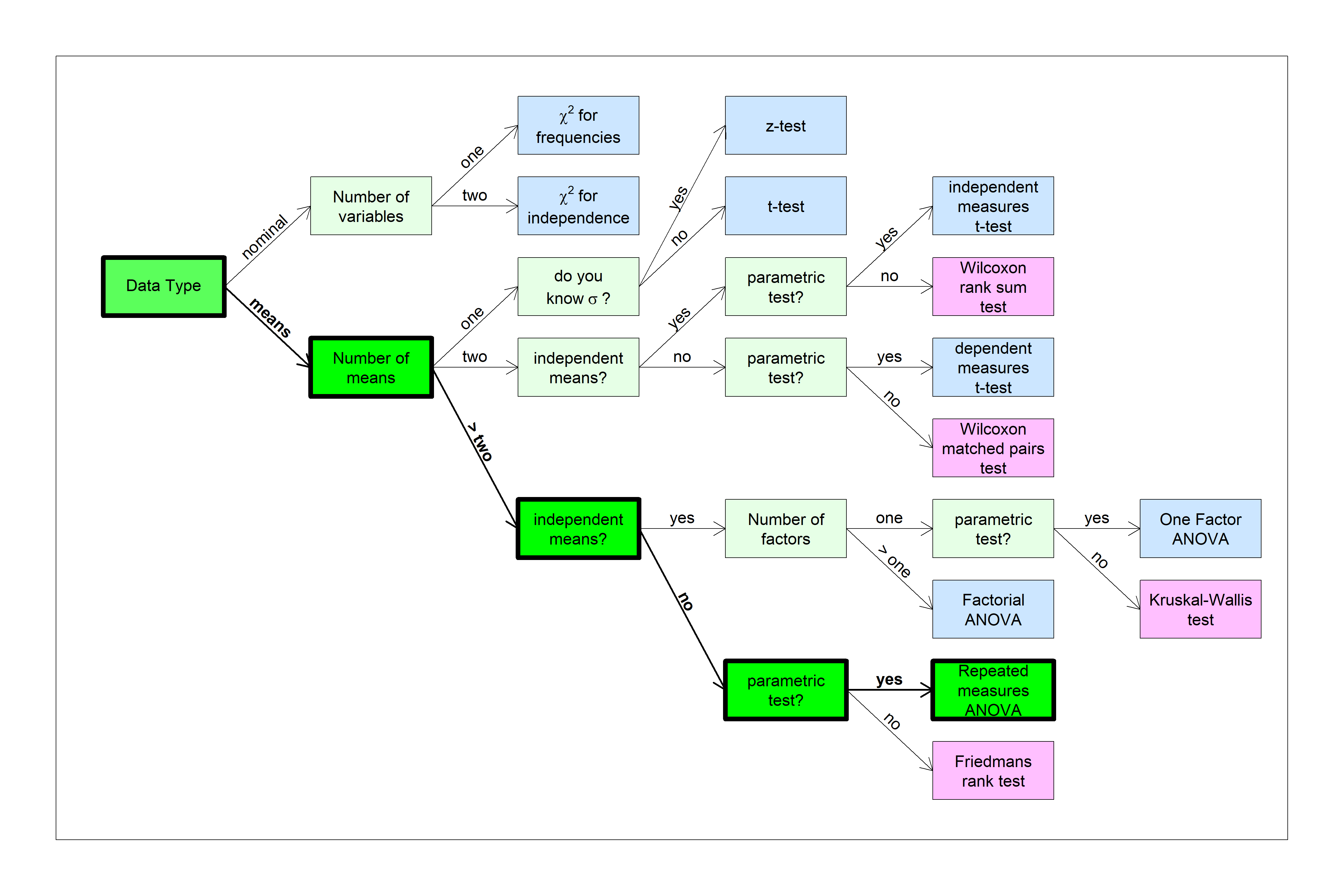
You can find this test in the flow chart here:
We’ll start with an example of a repeated measures t-test and build on that.
19.1 Review: Dependent measures t-test
Suppose you want to see if a specific exercise program affects body weight. You find 6 subjects and measure their weights (in kg) before the program and after three months. You can load in the (fake) data yourself in the course website:
data1 <- read.csv('http://courses.washington.edu/psy524a/datasets/SubjectExerciseANOVATtestdependent.csv')Some of these notes are based on the website (https://statistics.laerd.com/) which has some nice examples at the level appropriate for our class. The example in this chapter comes from (https://statistics.laerd.com/statistical-guides/repeated-measures-anova-statistical-guide-2.php)
A dependent (paired) t-test is equivalent to computing the difference between the two measurements for each subject and then running a one-sample t-test on those differences. Here’s a table of the results with the column of differences (after - before):
| Before | After Three Months | D |
|---|---|---|
| 45 | 50 | 5 |
| 42 | 42 | 0 |
| 36 | 41 | 5 |
| 39 | 35 | -4 |
| 51 | 55 | 4 |
| 44 | 49 | 5 |
Here’s how to run a dependent measures t-test on this data in R:
x <- data1$afterthreemonths
y <- data1$before
t.test.out <- t.test(x,y,paired = T,alternative = 'two.sided')
sprintf('t(%d) = %5.4f, p = %5.4f',t.test.out$parameter,t.test.out$statistic,t.test.out$p.value)
## [1] "t(5) = 1.6425, p = 0.1614"19.2 Repeated measures with more than two levels
What if we want to measure each subject again after six months? This requires measuring the differences between means across three different groups. ANOVA!
Unfortunately, while a dependent measures t-test is easier to compute than an independent measures t-test, a dependent measures ANOVA (often called within subjects or repeated measures ANOVA) is actually a little more complicated than the standard independent measures ANOVA.
Here’s how to load in the new data set from the course website:
data2 <- read.csv('http://courses.washington.edu/psy524a/datasets/SubjectExerciseANOVAdependent.csv')This data is stored in ‘long format’, where each row in the table corresponds to a different observation as opposed to ‘wide format’ where each row corresponds to a subject.
With long format, the first column, ‘subject’, determines the subject for the observation. The second column ‘time’ determines the condition for that observation. You’ll see that each subject has three observations, consistent with the repeated measures design:
| Subject | Time | Weight |
|---|---|---|
| S1 | before | 45 |
| S1 | after three months | 50 |
| S1 | after six months | 55 |
| S2 | before | 42 |
| S2 | after three months | 42 |
| S2 | after six months | 45 |
| S3 | before | 36 |
| S3 | after three months | 41 |
| S3 | after six months | 43 |
| S4 | before | 39 |
| S4 | after three months | 35 |
| S4 | after six months | 40 |
| S5 | before | 51 |
| S5 | after three months | 55 |
| S5 | after six months | 59 |
| S6 | before | 44 |
| S6 | after three months | 49 |
| S6 | after six months | 56 |
Long format may seem inefficient, but it’s a very convenient way to store your results, especially for complicated experimental designs. This way, every time you acquire a new measurement, you just add a new row to your data with the fields determining exactly which condition/subject the data came from. Most of the functions in R are designed for long format. t.test is an exception since it takes in ‘x’ and ‘y’ variables, but t.test can also accept data in long format.
19.2.1 Converting long format to wide
Sometimes it’s useful to see your results in ‘wide’ format, where each row is a subject. This can be done with R using a variety of functions. Here’s how to convert to wide format with the reshape function. You have to tell it the subject variable idvar = "subject" and the independent variable timevar = "time":
The data in wide format looks like this:
| Subject | Before | After Three Months | After Six Months |
|---|---|---|---|
| S1 | 45 | 50 | 55 |
| S2 | 42 | 42 | 45 |
| S3 | 36 | 41 | 43 |
| S4 | 39 | 35 | 40 |
| S5 | 51 | 55 | 59 |
| S6 | 44 | 49 | 56 |
19.2.2 As an independent measures ANOVA
Let’s first pretend that this is an independent measures design and run the ANOVA that way, ignoring the ‘subject’ field. We’ll also pull out the SS’s, MS’, and df’s from the table
## Analysis of Variance Table
##
## Response: weight
##           Df Sum Sq Mean Sq F value Pr(>F)
## time       2 143.44  71.722  1.5036  0.254
## Residuals 15 715.50  47.700
SS_between <- anova.out.1$`Sum Sq`[1]
df_between <- anova.out.1$Df[1]
MS_between <- anova.out.1$`Mean Sq`[1]
SS_within <- anova.out.1$`Sum Sq`[2]
df_within <- anova.out.1$Df[2]
MS_within <- anova.out.1$`Mean Sq`[2]
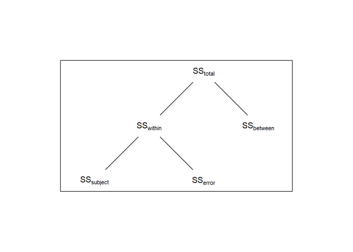
SS_total = SS_between+SS_within # remember?Remember, for a 1-factor ANOVA like this breaks down the total sums of squares so that
\[SS_{total} = SS_{between} + SS_{within}\]
Here, \(SS_{between}\) = 143.4444 reflects the variability across the ‘time’ factor, and \(SS_{within}\) = 715.5 is the variability within each level of time.
You wouldn’t want to analyze a repeated measures design this way because you wouldn’t be taking into account the variability in weights across the subjects. Treated as an independent measures ANOVA, this variability between subjects is part of \(SS_{within}\) (or ‘Residuals’ in R’s output).
Thus, for the denominator of the ANOVA for a repeated measures design we only want the component of \(SS_{within}\) that’s not associated with the variability across subjects. This is done by breaking down \(SS_{within}\) into two components: one component associated with within-subject variability, called \(SS_{subject}\) and the remaining variability called \(SS_{error}\):
In repeated-measures ANOVA we account for this by partitioning the within-group variability and removing the component, \(SS_{subject}\), associated with differences between subjects. This will make the denominator of the F-test smaller, and therefore the F-statistic larger.
We can calculate \(SS_{subject}\) in R by doing something a little weird - we’ll run another one-factor ANOVA, but this time with ‘subject’ as our factor. We’ll pull out the SS and Df from this analysis and call them \(SS_{subject}\) and \(df_{subject}\). This ANOVA estimates how much subjects differ after averaging across the time conditions.
## Analysis of Variance Table
##
## Response: weight
##           Df Sum Sq Mean Sq F value   Pr(>F)
## subject    5 658.28 131.656  7.8731 0.001706 **
## Residuals 12 200.67  16.722
## ---
## Signif. codes: 0 '***' 0.001 '**' 0.01 '*' 0.05 '.' 0.1 ' ' 1The p-value isn’t important here - it’s just telling us the significance of the variability across the the subjects’ weights after averaging across the three time conditions.
19.2.3 The denominator for the repeated measures ANOVA: \(SS_{error}\)
\(SS_{subject}\) is the sums of squared deviation of each subject from the grand mean, and is exactly the source of variability that we want to remove from our analysis.
For repeated measures ANOVA we do this by literally subtracting \(SS_{subject}\) from \(SS_{within}\) in the original independent measures ANOVA. We call this new sums of squared \(SS_{error}\)
\[SS_{error} = SS_{within} - SS_{subject}\]
which, for our example is:
## [1] 57.22222\(SS_{error}\) will serve as the sums-of-squares for the denominator for the repeated-measures ANOVA. To calculate \(MS_{error}\) we need to divide by the degrees of freedom for \(SS_{error}\). This is done in the same way as for sums-of-squared error:
\[df_{error} = df_{within} - df_{subject}\]
Which is, for our example:
The new denominator is:
## [1] 5.722222The F-statistic for the repeated measures uses the \(MS_{betweeen}\) from the original independent measures ANOVA for the numerator, but instead uses \(MS_{error}\) for the new denominator:
## [1] 12.53398Finally the p-value is calculated using the appropriate degrees of freedom:
## [1] 0.001885591After removing the variability due to differences between subjects, the error term becomes smaller, which increases the F-statistic.
19.3 Repeated measures ANOVA with R
The lm function that we used for independent measures ANOVA isn’t well set up for repeated measures designs. There are a few packages out there that can. I’m going to use the most general version, called lmer from the lme4 package. For reasons we’ll discuss later, we also have to include the lmerTest package because the creators of lmer are uncomfortable with providing p-values - again more on that later when we get into linear regression.
Once you have the packages installed, the use of lmer is much like it was for lm where we define the ‘model’ as weight ~ time. But now we have to tell the function which factor defines our subject with + (1|subject). The term (1|subject) is telling lm to allow each subject to have their own baseline weight - technically called a ‘random intercept’ for each subject. More on that later in the ‘Linear Mixed Models’ chapter.
## Type III Analysis of Variance Table with Satterthwaite's method
##      Sum Sq Mean Sq NumDF DenDF F value   Pr(>F)
## time 143.44  71.722     2    10  12.534 0.001886 **
## ---
## Signif. codes:  0 '***' 0.001 '**' 0.01 '*' 0.05 '.' 0.1 ' ' 1
You should recognize the SS, MS, df F and p-value from the analysis that we did by hand.
Don’t worry about the ‘Satterthwaite’s method’ thing for now. It’s a way of dealing with unbalanced designs. We’ll get into this once we’ve learned more about linear regression.
Here’s how to pull out the values in the output to make an APA formatted string:
sprintf('F(%g,%g) = %5.4f, p = %5.4f',
        anova.out.3$NumDF,anova.out.3$DenDF,anova.out.3$`F value`,anova.out.3$`Pr(>F)`)
## [1] "F(2,10) = 12.5340, p = 0.0019"19.4 Effect size for repeated measures ANOVA
19.4.1 Partial Cohen’s f
For any F-test, you can always calcuate Cohen’s f using our formula that uses the F-statistic and the two degrees of freedom. For the repeated measures ANOVA it’s called partial Cohen’s f (\(f_p\)):
\[f_p = \sqrt{F\frac{df_{between}}{df_{error}}}\]
With R using the ouput from anova(lmer... above:
partial_cohens_f <- sqrt(anova.out.3$`F value`*anova.out.3$NumDF/anova.out.3$DenDF)
cat(sprintf('Partial Cohens f: %0.2f',partial_cohens_f))
## Partial Cohens f: 1.58Calculating by hand:
\[f_p = \sqrt{12.53\frac{2}{10}} = 1.58\]
19.4.2 Partial eta-squared
Using the formula relating \(\eta^2\) to Cohens’f but using partial Cohen’s f, you can calculate partial eta-squared:
\[ \eta_p^2 = \frac{f_p^2}{1 + f_p^2} \] With a little algebra you can show that:
\[ \eta_p^2 = \frac{SS_{between}}{SS_{total}-SS_{subject}} \]
Compare this to the regular eta-squared (\(\eta^2\)) for the independent measures ANOVA:
\[ \eta^2 = \frac{SS_{between}}{SS_{total}} \]
You can see how this is similar to the calculation of \(MS_{error}\) for the repeated measures ANOVA:
\[ SS_{error} = SS_{within} - SS_{subject} \] Subtracting out \(SS_{subject}\) from the denominator for the repeated measures ANOVA results in subtracting out \(SS_{subject}\) from the denominator for partial eta-squared.
For repeated-measures ANOVA we typically report partial \(\eta_p^2\) which removes variability due to subjects from the denominator.
For our example:
\[\eta_p^2 = \frac{143.44}{858.94 - 658.28} = 0.71 \] The conventional interpretation for partial eta-squared is that .01 is small, .06 is medium and .14 is large. Our result would be considered to have a large effect size.
19.5 Power with repeated measures ANOVA
For any F-test, power can be calculated using pwr.f2.test with the Cohen’s F calculated from the formula with F’s and degrees of freedom. Using the ouptut of anova(lmer..., the observed power is:
power.anova.out <- pwr.f2.test(u = anova.out.3$NumDF,v = anova.out.3$DenDF,f2 = partial_cohens_f^2,sig.level = .05)
sprintf('Observed power: %5.4f',power.anova.out$power)
## [1] "Observed power: 0.9942"19.6 Sphericity
In this chapter we used the function lmer which is fitting what’s called a ‘mixed-effects’ model. This is a topic of a later chapter, but for now, for a balanced design and some assumptions about ‘random slopes’ and covariance structures, the classical way of computing repeated ANOVAs shown in this chapter will give you the same answer as treating it as a ‘mixed effects’ model.
However, by fitting this is as a mixed effect model with lm, we don’t have to worry about correlations between repeated measurements, so we don’t require correction for something called ‘sphericity’. But you will come across the issue of sphericity in older publications.
For this reason, mixed models are increasingly preferred over classical repeated-measures ANOVA.
Classical repeated-measures ANOVA requires an additional assumption called sphericity. Sphericity means that the variances of the differences between all pairs of repeated measurements are equal. Violations of this assumption cause the F-statistic to be too large, leading to inflated Type I error rates.
A common test for this assumption is Mauchly’s test of sphericity. If sphericity is violated, adjustments such as the Greenhouse–Geisser or Huynh–Feldt corrections modify the degrees of freedom of the F-test.
19.7 Apriori contrasts for repeated measures ANOVA
There isn’t a consensus on how Apriori and post hoc comparisons should be made with the repeated measures ANOVA. Since the difference between repeated measures and independent measures ANOVAs is the denominator, or ‘error’ term, you’d think that contrasts for repeated measures ANOVA would be the same as for independent, except that you’d use \(MS_{error}\) instead of \(MS_{within}\) in the denominator. However, apparently, this approach is too sensitive to violations of the assumption of sphericity.
Instead, when comparing two means, statisticians (for example Howell) suggest that you simply run t-tests (or ANOVAS) on each pair of means. These tests will only use a subset of the data for the denominator which gives you less power (fewer degrees of freedom in the denominator), but will be less biased due to issues with sphericity. Of course, you will also have to correct for familywise error using your favorite method, like Bonferroni.