Chapter 5 The Central Limit Theorem

In science, we are typically interested in the properties of a certain population, like, for example, the average height of men in a population. But sampling the entire population is usually impossible. Instead, we obtain a random sample from the population and hope that the mean from this sample is a good estimate of the population mean. How well does a sample mean represent the population mean?

The mean is an unbiased statistic, which means that a typical sample mean won’t be on average higher or lower than the population mean. But how close is a typical sample mean to the population mean? You probably have the intuition that this answer depends on the size of the sample. The larger the sample size, the closer the mean of your typical sample will be to the population mean. For example, it’s not too unusual to meet a man that is 6 foot 2 inches. But a room full of 25 men with average of 6 foot 2 would be surprising. Unless you’re in Holland.

The Central Limit Theorem is a formal description of this intuition. It’s a theorem that tells you about the .

5.1 The sampling distribution of the mean

Let’s take a moment to think about that term “distribution of sample means”. Every time you draw a sample from a population, the mean of that sample will be different. Some means will be more likely than other means. So it makes sense to think about the means drawn from a population as having their own distribution. This distribution is called the . The Central Limit Theorem tells us how the shape of the sampling distribution of the mean relates to the distribution of the population that these means are drawn from.

To define some terms, if samples from a population are labeled with the variable \(X\), we define the parameters of mean as \(\mu_{x}\) and the standard deviation as \(\sigma_{x}\). Remember, the greek letter is the parameter, and the subscript is the name of the thing that we’re talking about.

Now consider the sampling distribution of the mean. You know that sample means are written as \(\bar{x}\). Using the same notation, the sampling distribution of the mean has its own mean, called \(\mu_{\bar{x}}\), and its own standard deviation, called \(\sigma_{\bar{x}}\).

There are three parts to the Central Limit Theorem:

The sampling distribution of the mean will have the same mean as the population mean. Formally, we state: \(\mu_{\bar{x}} = \mu_{x}\).

This just means what I said earlier, that the mean is unbiased, so that sample means will be, on average, equal to the population mean.

For a sample size \(n\), the standard deviation of the sampling distribution of the mean will be \(\sigma_{\bar{x}} = \frac{\sigma_{x}}{\sqrt{n}}\)

The name for \(\sigma{\bar{x}}\) is sometimes shortened to the standard error of the mean, and sometimes shortened even more to ‘s.e.m.’ or even just ‘SE’.

This is a formalization of the intuition above. Since \(\sqrt{n}\) is in the denominator, it means that as your sample size gets bigger, the standard deviation of the distribution of means, \(\sigma_{\bar{x}}\), gets smaller. So as you increase sample size, any given sample mean will be on average closer to the population mean.

The sampling distribution of the mean will tend to be close to normally distributed. Moreover, the sampling distribution of the mean will tend towards normality as (a) the population tends toward normality, and/or (b) the sample size increases.

This last part is the most remarkable. It means that even if the population is not normally distributed, the sampling distribution of the mean will be roughly normal if your sample size is large enough.

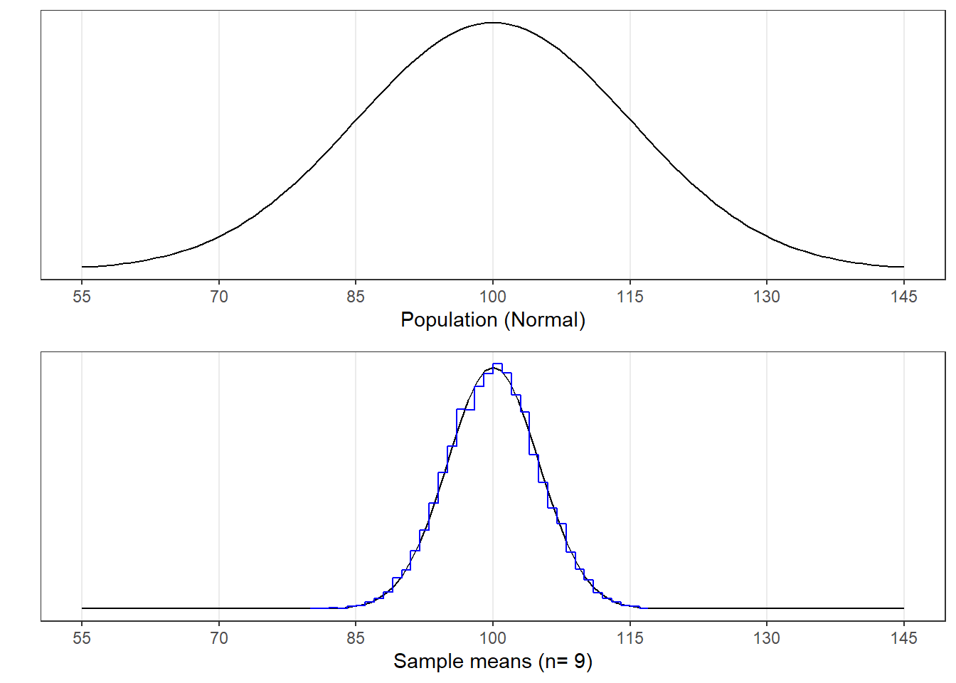
Below is the results of a simulation demonstrating the Central Limit Theorem.

The graph on the top is the population distribution, which for this example is normal with a mean of \(\mu_{x} = 100\) and a standard deviation of \(\sigma_{x} = 15\). The simulation ran 10^{4} samples of size n=9.

In the bottom graph in blue you can see a histogram of the means from these samples. Drawn on top of the histogram is the expected normal distribution of means according to the Central Limit Theorem:

\(\mu_{\bar{x}} = \mu_{x} = 100\) and \(\sigma_{\bar{x}} = \frac{\sigma_{x}}{\sqrt{n}} = \frac{15}{\sqrt{9}} = 5\)

You can see that the smooth curve matches the distribution of actual means. The mean of sample means in this simulation is 99.97 and the standard deviation of the means is 5.01 - pretty close to what’s expected from the Central Limit Theorem.

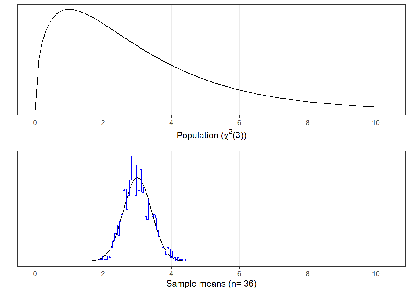
In this second demonstration we’ll draw from a population that is clearly not normally distributed:

This time the population is a ‘Chi-squared’ (\(\chi^{2}\)) distribution, which will show up later. The population has a mean of 3 and standard deviation of 2.4495.

Like before, the blue histogram in the bottom graph shows the distribution of 1000 means of sample size 36 from this skewed population distribution. Notice that sample means have a nice, symmetric normal-looking distribution.

The Central Limit Theorem predicts that the distribution of means should be roughly normal with a mean of \(\mu_{\bar{x}} = \mu_{x} = 3\) and a standard deviation of \(\sigma_{\bar{x}} = \frac{\sigma_{x}}{\sqrt{n}} = \frac{2.4495}{\sqrt{36}} = 0.4082\)

In this simulation, the mean of these means is 2.99 which is close to the population mean, and a standard deviation of 0.4125, which is close to what’s expected from the Central Limit Theorem. Like the first example, the smooth curve in the bottom graph is a normal distribution with the mean and standard deviation expected from the Central Limit Theorem. It clearly matches the distribution of sample means from the simulation.

The Central Limit Theorem is powerful because, as we’ve learned from previous chapters, if you know that a distribution is normal, and you know its mean and standard deviation, then you know everything about this distribution.

Next we’ll work through some examples to show how we can use the Central Limit Theorem to make inferences about the population that a sample is drawn from.

5.2 Examples

5.2.1 Example 1

What is the probability that a mean drawn from a sample of 25 IQ scores will exceed 103 points?

IQs are normalized to have a mean of 100 and a standard deviation of 15. From the Central Limit Theorem, a mean from a sample size of 25 will come from its own distribution with a mean of 100 and a standard deviation of \(\frac{15}{\sqrt{25}} = 3\)

We can then use R’s ‘pnorm’ function to find the area from this normal distribution above a mean of 103:

mu <- 100
sigma <-15
X <- 103
sem <- sigma/sqrt(n)
p <- 1-pnorm(X,mu,sem)
p

## [1] 0.1586553

So there is about a 16% chance that we’ll draw a mean IQ of 103 or higher.

5.2.2 Example 2

In the last chapter we had examples using the fact that the average height of women in the world globally is 63 inches, with a standard deviation of 2.5 inches. Consider the mean height of 100 randomly sampled women this population. For what mean height will 5% of the means fall above?

Answer:

With a sample size of 100, the Central Limit Theorem states that the means will be distributed with a mean of 63 inches and a standard deviation of \(\frac{2.5}{\sqrt{100}} = 0.25\) inches. We can find the height for which 5% falls above using R’s ‘qnorm’ function to find the height for which the area below is 0.95:

mu <- 63
sigma <- 2.5
sem <- sigma/sqrt(n)
n <- 100
p <- 1-.05
x <- qnorm(p,mu,sem)
sprintf('The height for which %g%% of the means falls above is %5.2f inches.',100*(1-p),x)

## [1] "The height for which 5% of the means falls above is 63.41 inches."

Always check your answer to see if it makes sense. 63.41 inches is greater than the population mean of 63 inches, which makes sense since this mean is the cutoff for the upper 5%.

5.2.3 Example 3

From the survey, the mean height of the 122 women in Psych 315 had a height of 64.7 inches. If we assume that the women in Psych 315 are drawn randomly from the world population from Example 2, what is the probability of obtaining a mean this high or higher by chance?

Answer:

From the Central Limit Theorem, the means will be distributed with a mean of 63 inches and a standard deviation of \(\frac{2.5}{\sqrt{122}} = 0.23\) inches. The probability of obtaining a mean of 64.7 or higher can be calculated from R’s ‘pnorm’ function. Here’s the code, which loads in the survey data:

mu <- 63
sigma <- 2.5

survey <- read.csv("http://www.courses.washington.edu/psy315/datasets/Psych315W21survey.csv")

women.height <- na.omit(survey$height[survey$gender=="Woman"])
x <- mean(women.height)
n <-length(women.height)
sem <- sigma/sqrt(n)

p <- 1-pnorm(x,mu,sem)  #sem from problem 2
sprintf('The probability of drawing a mean of %5.2f or higher is %g',x,p)

## [1] "The probability of drawing a mean of 64.70 or higher is 2.4869e-14"

This is an extremely low probability. That’s because with a standard error of the mean of \(\sigma_{\bar{x}} = 0.23\), a mean of 64.7 is \(\frac{64.7 - 63}{0.23} = 7.53\) standard deviations above the population mean of 2.5.

What does this mean about the women in Psych 315? They seem to be impossibly tall. This is true assuming that these students are randomly sampled from the world’s population. So logically, there seems to be something wrong with this assumption. It is more likely that this assumption is false, and the true population that we’re drawing from has a mean taller than 63 inches.