Chapter 8 Confidence Intervals and Effect Size

The last example in the last chapter we tested the hypothesis that the heights of the men in Psych 315 was significantly different from 70 inches. We calculated that \(n = 29\), \(\bar{x} = 70.3103\), \(s = 3.1521\) and \(s_{\bar{x}} = 0.5853\).

From these values, the t-statistic was found to be:

\(t = \frac{(\bar{x} - \mu_{H0})}{s_{\bar{x}}} = \frac{70.31-70}{0.5853} = 0.5302\)

and the p-value was:

\(p = 0.6002\)

The t-distribution, like the z-distribution, is the distribution of scores that you’d expect from an experiment if the null hypothesis is true. That’s why it’s centered around zero. On average your observed mean will be somewhere around the null hypothesis mean.

Let’s look at where our t-statistic (t = 0.5302) falls compared to the rejection region (using a two-tailed test with \(\alpha = 0.05\)):

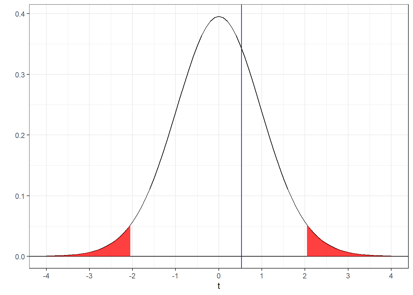
You can see why we failed to reject \(H_{0}\). Our t-statistic (blue line) falls outside the rejection region (red tails).

With a little algebra we can rearrange the above equation to:

\[ \bar{x} = \mu_{H_0} + s_{\bar{x}} \times t \] This equation says that if the null hypothesis is true, then the expected distribution of means is shaped like a t-distribution scaled by \(s_{\bar{x}} = 0.5853\) and centered at \(\mu_{H_0}\). Here’s a plot of the distribution of means expected if the \(H_{0}\) is true. Instead of shading the outer 5% in red, I’ve shaded the middle 95% in blue:

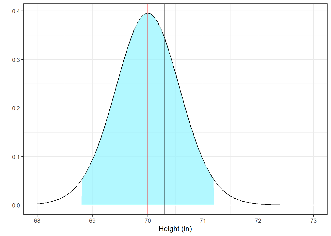This looks just like the picture for the t-distribution, but shifted into our measured value of inches. Again you can see how the observed mean of 70.3103 falls with respect to the middle 95% of the distribution of means.

Now, let’s forget about the null hypothesis. Instead, let’s assume that our observed mean is the actual center of the population distribution. If we do this, then the expected distribution of means will look like the picture above, but will instead be centered at \(\overline{x}\) = 70.3103. The confidence interval can therefore be defines as:

\[ CI = \bar{x} \pm s_{\bar{x}} \times t \]

This figure shows the 95% confidence interval for our example. It looks like the previous figure but with the scaled t-distribution now centered at \(\bar{x}\). Again, the null hypothesis is shown as a vertical red line.

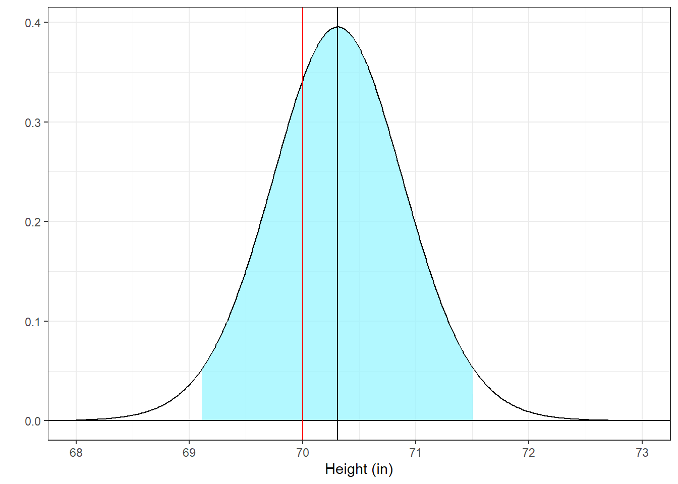
Assuming that \(\overline{x}\) is the true population mean, then we expect the means to fall in the blue shaded region 95% of the time, so we call this region the 95% confidence interval.

Notice that we can make the same decision about rejecting \(H_{0}\) by comparing where \(H_{0}\) falls with respect to the confidence interval. If \(H_{0}\) falls inside the confidence interval, we fail to reject \(H_{0}\).

Using R, we can calculate this interval by using qt to find the values of t covering the middle 95% and shifting and scaling these values by \(s_{\bar{x}}\) and \(\bar{x}\):

survey <- read.csv("http://www.courses.washington.edu/psy315/datasets/Psych315W21survey.csv")

alpha <- .05
x <- na.omit(survey$height[survey$gender == "Man"])
t.test.out <- t.test(x,mu = 70)
m <- mean(x)
n <- length(x)
sem <- sd(x)/sqrt(n)
df <- n-1
tRange <- qt(c(alpha/2,1-alpha/2),df)   
CI <- m + sem*tRange  
round(CI,2)

## [1] 69.11 71.51

This is our 95% confidence interval. It matches the values that came out of t.test which can be found in t.test.out$conf.int

t.test.out$conf.int

## [1] 69.11134 71.50935
## attr(,"conf.level")
## [1] 0.95

As we’re encouraged to move away from p-values, journals more commonly asking for confidence intervals because they don’t depend on a null hypothesis. But we can still use them to make our decision about rejecting \(H_{0}\). Again, we can therefore reject \(H_{0}\) if and only if the null hypothesis mean falls outside the confidence interval.

For this example 70 falls inside the confidence interval so we fail to reject \(H_{0}\). You can see this in the plot above where the vertical line marking the null hypothesis mean (70) falls inside the blue shaded region.

A nice thing about confidence intervals compared to p-values and t-statistics is that they are in the units of our measurement (inches for our example). And, for this reason, they give us our critical value for rejecting \(H_{0}\) in our measured units. We know that if your null hypothesis was either \(H_{0}: \mu = 69.11\) or \(H_{0}: \mu = 71.51\) - the lower and upper ranges of our confidence interval - our mean would be right on the border of rejecting, and therefore our p-value would be 0.05.

But, confidence intervals alone don’t tell us the statistical significance of the test, which is why we’re often asked to report both confidence intervals and p-values.

8.1 Effect Size

Remember, ‘statistical significance’, which is the p-value, is the probability that you’d obtain your observation given that \(H_{0}\) is true. But even though the word ‘significant’ sounds like ‘important’, at statistically significant result may not be that interesting. Here’s an example.

8.2 An Uninteresting Example

We’ll go back to IQ’s again so that we can use the simple z-test, but the idea holds for any hypothesis test.

Suppose you want to test the hypothesis that the IQ’s of college students is different from 100. You go and sample the entire undergraduate population at UW which in 2021 had an enrollment of 36206 students and find that the mean IQ of UW undergraduates is 100.25. With our sample size, the standard error of the mean is \(\frac{\sigma}{\sqrt{n}} = \frac{15}{\sqrt{36206}} = 0.0788\)

Our z-score is therefore:

\[ \frac{(\bar{x}-\mu)}{\sigma_{\bar{x}}} = \frac{(100.25 - 100)}{0.0788} = 3.1713\] Using R’s ‘pnorm’, our p-value for a two-tailed test is:

2*(1-pnorm(abs(3.1713)))

## [1] 0.001517583

We conclude that our mean of 100.25 is significantly different from 100 and that IQ’s of college students is significantly different from the general population.

But how excited can you be about a \(\frac{1}{4}\) of an IQ point difference? I don’t think it’s something you’d run out and tell your friends and send the result to Nature or something.

Of course, our results are statistically significant because our sample size is so large. To bend Archimedes, “Give me a sample size large enough and I can reject any \(H_{0}\)”. Technically this is only true if \(H_{0}\) is false, but it doesn’t have to be very false.

So the problem with p-values is that they don’t reflect the real size of the effect. The difference between the sample mean and the null hypothesis mean (100.25 - 100 = 0.25) is helpful, but it’s hard to interpret because it doesn’t take into account the variability in the population that we’re sampling from.

We need something sort of in between the p-value and the difference between means. This is the effect size. It’s defined as ‘Cohen’s d’, which looks like the formula for a z or t-score, but has the standard deviation in the denominator instead of the standard error of the mean:

\[ d = \frac{|\bar{x}-\mu_{hyp}|}{\sigma_{x}} \]

Or if you don’t know \(\sigma\):

\[ d = \frac{|\bar{x}-\mu_{hyp}|}{s_{x}} \]

Cohen’s d is the difference in the means in standard deviation units. For IQ’s, a mean IQ of 115 would have an effect size of d=1, since 115 is one standard deviation above the mean. For our example:

\[ d = \frac{|\bar{x}-\mu_{hyp}|}{\sigma_{x}} = \frac{|100.25 - 100|}{15} = 0.0167 \] Our difference in means is very small compared to the standard deviation of the population.

For the social sciences, almost all textbooks define the size of Cohen’s d to be:

Table 8.1: Cohen’s d

small	.2
medium	.5
large	.8

These values are a rough guide. We’re allowed to embellish - for our IQ example it’s fair to say that we have a ‘very small’ or ‘teeny weeny’ effect size.

There are two main advantages effect size. The first is that it doesn’t depend on the sample size (although it does get more reliable with increasing sample size), and second, it’s in standardized units. This means that effect sizes can be compared across experiments that have different units and sample sizes.

8.3 Summary

We now have four ways of telling people about the size of our results. First, there’s simply the difference between our observed mean and null hypothesis mean. Then there is the p-value, the confidence interval, and the effects size. Each has their own advantages and disadvantages. The following table summarizes the attributes of each:

Table 8.2:

	Statistical significance	Real units	Compare across experiments	Requires \(H_0\)	Decision about \(H_0\)
Difference of Means	No	Yes	No	Yes	No
p-value	Yes	No	No	Yes	Yes
Confidence Interval	Yes (sort of)	Yes	No	No	Yes
Effect Size	No	No	Yes	Yes	No

Note that ‘Yes’ or ‘No’ aren’t necessarily ‘Pros’ or ‘Cons’. For example, the attribute ‘in real units’ is useful because it’s easily interpreted, but can’t easily be used to compare across experiments.

I’ve put ‘sort of’ for confidence intervals giving statistical significance because, as we discussed, you can see if your confidence interval includes the null hypothesis mean to make a binary decision, but it doesn’t give you quantitative measure like the p-value.