Chapter 23 Linear Mixed Models
23.1 Using lmer for a Repeated Measures Design
In the previous chapter Linear Models we covered how to run one and two factor ANOVAs with R’s ‘lm’ function. All of the examples in that chapter were independent measures designs, where each subject was assigned to a different condition. Now we’ll move on to experimental designs with ‘random factors’ like repeated measures designs and ‘mixed models’ that have both within and between subject factors. R’s ‘lm’ function can’t handle design with random factors, so we’ll use the most popular function ‘lmer’ from the ‘lme4’ package. Go ahead and install it if you haven’t already.
23.2 Example: Effect of Exercise over Time on Body Weight
We’ll start with the first example from the Repeated Measures ANOVA chapter. The first example was the study of exercise over time on weight (in kg). In this example, 6 subjects’ weights were measured over 3 points in time: “before”, “after three months”, and “after six months” since starting the exercise program.
First we’ll load in the data and take a look:
weightData<-
  read.csv("http://www.courses.washington.edu/psy524a/datasets/SubjectExerciseANOVAdependent.csv")

head(weightData)
## subject time weight
## 1 S1 before 45
## 2 S1 after three months 50
## 3 S1 after six months 55
## 4 S2 before 42
## 5 S2 after three months 42
## 6 S2 after six months 45The advantage of a repeated measures design is that we can subtract out the individual differences in each subject’s weight. ‘subject’ is a ‘random effect factor’, as opposed to ‘time’, which is a ‘fixed effect factor’. A random effect factor has many possible levels, but the experiment only sampled a subset of them. By defining a factor as a random effect factor, you are seeing if your results generalize across all levels of that factor. ‘subject’ is a random effect factor because you have sampled a subset of subjects for your experiment, and you want to make conclusions about the entire population of subjects, not just the ones that you’ve sampled. Conclusions made from fixed effect factors can only be attributed to the specific levels that you included in your experiment.
In the context of ANOVA, we dealt with subject as a repeated measure factor by subtracting out the individual differences in weight across subjects by calculating \(SS_{subjects}\) and subtracting that from \(SS_{within}\). Mathematically it makes sense - you get to see how the systematic error is taken away from the SS for the denominator of the F-test, thereby increasing F and decreasing your p-value.
Another way to think about accounting for individual differences in weight is to add a regressor for each subject to your model so that each subject gets its own free parameter, called an ‘intercept’. Here’s how to use lmer to fit a regression model to the exercise data:
The first part of the model uses the same conventions as ‘lm’. \(weight ~ time\) should look familiar; we’re predicting weight as a function of the factor, time. The new part is the stuff in parentheses which defines the random effect variable. \((1|subject)\) means that we’re going to allow for an intercept for each subject. When we pass the output of lmer into ‘anova’ you’ll see the same results as in the Repeated Measures ANOVA chapter:
## Type III Analysis of Variance Table with Satterthwaite's method
##      Sum Sq Mean Sq NumDF DenDF F value   Pr(>F)
## time 143.44  71.722     2    10  12.534 0.001886 **
## ---
## Signif. codes:  0 '***' 0.001 '**' 0.01 '*' 0.05 '.' 0.1 ' ' 1
Let’s use the ‘coef’ function to look at the values (coefficients) that best fit the data:
## $subject
##    (Intercept) timeafter three months timebefore
## S1    53.54595              -4.333333  -6.833333
## S2    46.85020              -4.333333  -6.833333
## S3    43.98059              -4.333333  -6.833333
## S4    42.06752              -4.333333  -6.833333
## S5    58.32864              -4.333333  -6.833333
## S6    53.22711              -4.333333  -6.833333
##
## attr(,"class")
## [1] "coef.mer"
This looks different than the coefficients for the between subjects ANOVA discussed in the Linear Models chapter. Here there is a row for every subject. This is because with a repeated measure design like this, every subject gets their own ‘intercept’, which allows for each subject’s weight to vary overall. The other two coefficients are the same across subjects. That’s because ‘time’ is a fixed effect variable, so it affects all subjects the same way.
These coefficients are in the same form as for the independent measures ANOVA. Alphabetically, ‘after six months’ comes first, so this is the first regressor.
The two columns correspond to the difference between the ‘after six months’ condition
For a simple example like this, it turns out that we could have used the old ‘lm’ function to allow for a different parameter for each subject. This is simply done by letting our model be \(weight ~ time + subject\). Note the lack of interaction in the model:
## Analysis of Variance Table
##
## Response: weight
##           Df Sum Sq Mean Sq F value    Pr(>F)
## time       2 143.44  71.722  12.534  0.001886 **
## subject    5 658.28 131.656  23.008 3.461e-05 ***
## Residuals 10  57.22   5.722
## ---
## Signif. codes:  0 '***' 0.001 '**' 0.01 '*' 0.05 '.' 0.1 ' ' 1
We get the same F and p-values for the effect of time. We also get a measure of the differences in weights across subjects, which we don’t care about. You can see how there’s confusion about the definition of a random factor. Using ‘lm’ we’re thinking of both time and subject as fixed factors, but with ‘lmer’ we’re thinking of time as fixed but subject as random. But the results turn out the same.
You’re now probably wondering why we have ‘lmer’ if we get the same thing using ‘lm’, treating all variables as fixed, and just ignoring the results from the variables we don’t care about. The reason is that ‘lmer’ can handle much more complicated situations that ‘lm’ can’t deal with. For example, mixed designs:
23.3 Mixed Design Example: Effect of Napping and Time on Perceptual Performance
A mixed-design has a mixture of independent and dependent (usually repeated) measures factors. The math behind mixed-designs are extensions of what we already know about independent and dependent measures, so although it sounds complicated, it’s not that bad. The simplest mixed design has one independent and one dependent factor. Here’s an example:
A former postdoc of mine, Sara Mednick, found that if you test the same subject on a texture discrimination task (finding a T amongst L’s) your threshold (in milliseconds) increases (gets worse) across sessions throughout the day (when testing at 9am, 12pm, 3pm and then 6pm). In her experiment, half of the subjects took a nap after the 12pm session.
This is a mixed design because it has one within-subjects factor and one between-subjects factor. The time of testing is the within-subjects factor (each subject was tested four times), and the napping condition (nap vs. no nap) is the between-subjects factor.
Let’s load in the data and take a peek:
napData<-read.csv("http://www.courses.washington.edu/psy524a/datasets/napXtimemixed.csv")
head(napData)
## subject sleep time threshold
## 1 S1 no nap 9am 151
## 2 S1 no nap 12pm 285
## 3 S1 no nap 3pm 180
## 4 S1 no nap 6pm 356
## 5 S2 no nap 9am 105
## 6 S2 no nap 12pm 179There are three independent factors: subject, sleep, and time. Subject is a random factor, sleep is a between subject factor and time is a within subject factor. The dependent factor is threshold.
Next we’ll use ‘summarySE’ from the ‘Rmisc’ library and ‘ggplot’ from the ‘ggplot2’ library to compile the data and make plot of the means and standard errors over time.
# reorder the levels for time
napData$time <- ordered(napData$time, levels = c( "9am","12pm","3pm","6pm"))
# get the means and standard errors
napData.summary <- summarySE(napData, measurevar="threshold", groupvars=c("sleep","time"))
ggplot(napData.summary, aes(x=time,y=threshold,colour = sleep, group = sleep)) +
geom_errorbar(aes(ymin=threshold-se, ymax=threshold+se), width=.2) +
geom_line() +
theme_bw() +
geom_point(size = 5)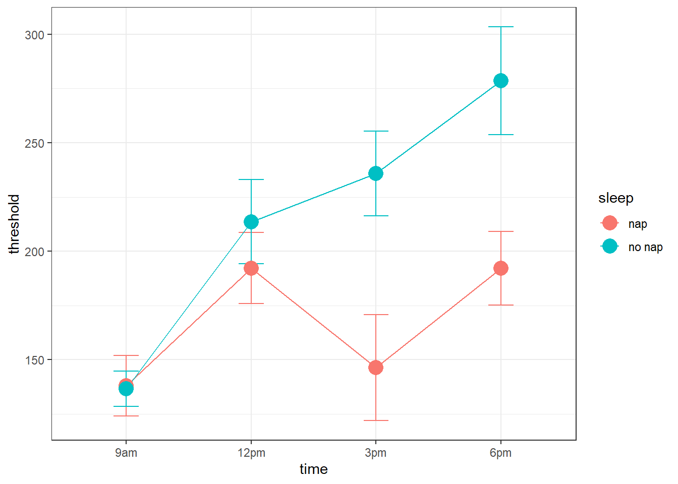 Notice how the thresholds decrease over time for the subject that didn’t get a nap, but when subjects took a nap after 12pm, thresholds dropped back down (and then climbed back up for the 6pm session).
Now we’ll fit the data with a linear model with the factors to see if there’s a significant effect of time, sleep and and interaction. The analysis is straightforward using lmer. The model is simply \(threshold ~ time*sleep + (1|subject)\). We don’t have to tell lmer which factor is between and which is within. It’s all apparent in the data.
## Type III Analysis of Variance Table with Satterthwaite's method
##            Sum Sq Mean Sq NumDF DenDF F value    Pr(>F)
## time        49950 16649.9     3    24 11.7345 6.277e-05 ***
## sleep       12497 12497.4     1     8  8.8079   0.01793 *
## time:sleep  15873  5290.9     3    24  3.7289   0.02482 *
## ---
## Signif. codes:  0 '***' 0.001 '**' 0.01 '*' 0.05 '.' 0.1 ' ' 1
The three hypothesis tests here - two main effects and an interaction - aren’t necessarily the most interesting set of tests for this experiment. Yes, there is a main effect of sleep, so thresholds without a nap are higher than with a nap. But there’s also an interaction between time and sleep, which makes the main effect of sleep more difficult to interpret. Another test we could run (it’d be an ariori test if we had thought of it before running the experiment) would be to look only at the 3pm and 6pm data. This can be done using the ‘subset’ function:
afternoonData <- subset(napData,time == "3pm" | time == "6pm")

lmer4.out <- lmer2.out  <- lmer(threshold ~ time*sleep + (1|subject),data = afternoonData)
anova(lmer4.out)
## Type III Analysis of Variance Table with Satterthwaite's method
## Sum Sq Mean Sq NumDF DenDF F value Pr(>F)
## time 9857 9857 1 8 4.3524 0.07043 .
## sleep 35846 35846 1 8 15.8281 0.00407 **
## time:sleep 13 13 1 8 0.0057 0.94192
## ---
## Signif. codes: 0 '***' 0.001 '**' 0.01 '*' 0.05 '.' 0.1 ' ' 1Here, consistent with the plot, for just the afternoon you can see that there’s a main effect for time (threshold go up between 3pm and 6pm), there’s a main effect of sleep (thresholds are higher without a nap), but no interaction between time and sleep. Note that running an analysis on a subset of the data is a little like running a simple effects analysis with ANOVAs.
23.4 Mixed Design Example: Effect of Donezepil on Test Scores
Suppose you want to test the efficacy of the Alzheimer’s drug, Donepezil on various cognitive tests. 8 subjects are divided into 2 groups, “without Donepezil”, and “with Donepezil”, and each subject is given 3 tests: “memory”, “reading”, and “verbal”. 8 subjects are divided into 2 groups, “without Donepezil”, and “with Donepezil”. Each subject repeats each test across 5 days.
This is a mixed design because ‘drug’ is a between subject factor and both ‘test’ and ‘day’ are within subject factors.
Let’s load in the data file and take a look:
drugData<-read.csv("http://www.courses.washington.edu/psy524a/datasets/DrugTestMixed.csv")
head(drugData)
## subject drug day test score
## 1 S1 without Donepezil Mon memory 45.74021
## 2 S2 without Donepezil Mon memory 69.44595
## 3 S3 without Donepezil Mon memory 34.52847
## 4 S4 without Donepezil Mon memory 32.22222
## 5 S1 without Donepezil Tue memory 37.61943
## 6 S2 without Donepezil Tue memory 84.60970Let’s not worry about the ‘day’ factor for now and plot the test scores across groups:
# get the means and standard errors
drugData.summary <- summarySE(drugData, measurevar="score", groupvars=c("drug","test"))

ggplot(drugData.summary, aes(x=test,y=score,colour = drug, group = drug)) +
  geom_errorbar(aes(ymin=score-se, ymax=score+se), width=.2) +
  geom_line() +
  theme_bw() +
  geom_point(size = 5)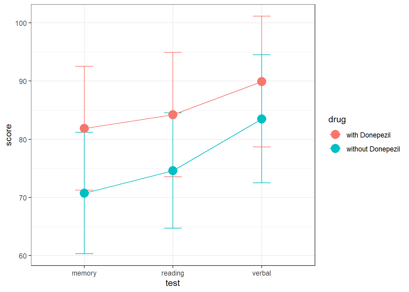
It looks like test scores are slightly higher with Donepezil, but the overlapping error bars mean that it might not be statistically significant. Also, there doesn’t look like there’s much difference across test scores. Let’s run the regression analysis, leaving out the interaction. We’ll use ‘(1|subject)’ as the random effect.
# Run the ANOVA
lmer5.out <- lmer(score ~ test + drug + (1|subject),data =drugData)
anova(lmer5.out)
## Type III Analysis of Variance Table with Satterthwaite's method
## Sum Sq Mean Sq NumDF DenDF F value Pr(>F)
## test 2275.24 1137.62 2 110 1.1939 0.3069
## drug 91.26 91.26 1 6 0.0958 0.7674As predicted from the graph, the effects of the drug are not statistically significant, nor is there a significant difference in scores across the tests.
To understand how the regression model fit the data, it helps to look at the best fitting coeficents, or beta weights:
## $subject
##    (Intercept) testreading testverbal drugwithout Donepezil
## S1    48.00598    3.103345     10.389             -9.056597
## S2   134.60783    3.103345     10.389             -9.056597
## S3    84.38692    3.103345     10.389             -9.056597
## S4    56.39305    3.103345     10.389             -9.056597
## S5    43.34021    3.103345     10.389             -9.056597
## S6   136.82312    3.103345     10.389             -9.056597
## S7    82.53079    3.103345     10.389             -9.056597
## S8    60.69966    3.103345     10.389             -9.056597
##
## attr(,"class")
## [1] "coef.mer"
The coeficients tell us how the model predicts each data point. Notice how using ‘(1|subject)’ as the random effect in lmer allows for a different intercept for each subject. However, the coeficients for the other levels are all the same. That’s because test and drug are fixed factors. We can use these coeficients to see the model predictions. Since ‘memory’ is the first level alphabetically in the test levels, the effects of the other levels are added to the ‘memory’ score. For example, subject S1, who is in the ‘without Donepezil’ group, has a predicted test score for ‘memory’ that is this subject’s intercept plus the effect of being in the ‘without Donepizil’ group:
\(48.006-9.0566 = 38.9494\)
This subject’s predicted score for the ‘reading’ group is this subject’s intercept plus the effect of being in the ‘without Donepizil’ group plus the effect of being in the ‘reading’ group:
\(48.006-9.0566+3.10335 = 42.0527\)
What about the ‘day’ factor? It turns out that there is a significant amount of learning across days in this (fake) data set. We can see this by plotting the test scores across days (averaging across the three tests) for each subject:
But what about ‘day’?
drugData.day.summary <- summarySE(drugData, measurevar="score", groupvars=c("day","subject"))
drugData.day.summary$day <- ordered(drugData.day.summary$day, levels = c("Mon","Tue","Wed","Thu","Fri"))
ggplot(drugData.day.summary, aes(x=day,y=score,colour = subject, group = subject)) +
geom_errorbar(aes(ymin=score-se, ymax=score+se), width=.2) +
geom_line() +
theme_bw() +
geom_point(size =3)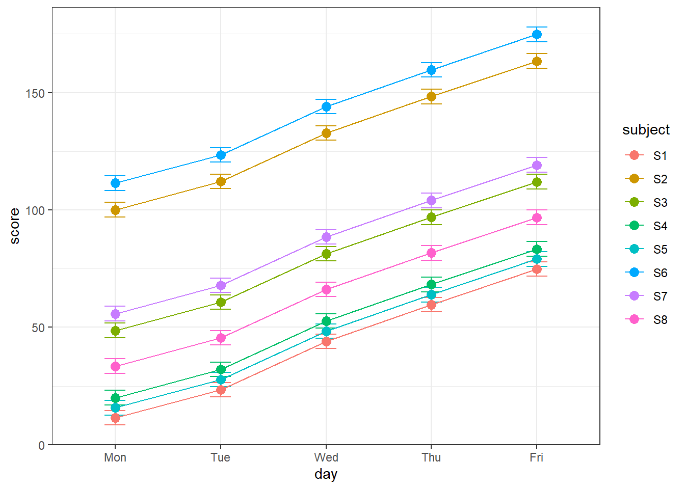 Can you see the improvement in scores across the week? ‘day’ is a random effect variable, since it’s a variable that influences our results but we’re not interested in it as part of our study. To account for it, we add five more parameters to the model: an intercept for each day by adding ‘(1|day)’ as a random effect:
## Type III Analysis of Variance Table with Satterthwaite's method
##       Sum Sq Mean Sq NumDF DenDF F value  Pr(>F)
## test 2275.24 1137.62     2   106  3.1775 0.04569 *
## drug   34.29   34.29     1     6  0.0958 0.76742
## ---
## Signif. codes:  0 '***' 0.001 '**' 0.01 '*' 0.05 '.' 0.1 ' ' 1
Now you can see that there is (barely) a significant difference across the three test scores. Note, however, that the results for the ‘drug’ factor hasn’t changed. This is because ‘drug’ is a between subject factor for both day and subject. So repeated measures across tests and day doesn’t help the test of drug. ‘subject’ as random effect variables only increases the power of the test for drug if each subject was tested both with and without the drug. Similarly, with ‘day’ as a random effect would only help the effect of drug if the drug was introduced across days.
One way to see how your model predicts the data is to plot the model’s prediction instead of the real data. An easy way to do this is to create a new data set from the old one, and replace the real data with the model predictions using R’s ‘predict’ function. Here’s how:
# copy the original data into a new data frame
predDrugData <- drugData

# replace the real dv 'score' with the predicted scores
predDrugData$score <- predict(lmer6.out)

# plot the data like we did before
predDrugData.day.summary <- summarySE(predDrugData, measurevar="score", groupvars=c("day","subject"))
predDrugData.day.summary$day <- ordered(predDrugData.day.summary$day, levels = c("Mon","Tue","Wed","Thu","Fri"))

ggplot(predDrugData.day.summary, aes(x=day,y=score,colour = subject, group = subject)) +
  geom_errorbar(aes(ymin=score-se, ymax=score+se), width=.2) +
  geom_line() +
  theme_bw() +
  geom_point(size =3)
It’s clear now how using subject and day affects the model predictions. Each day and subject contribute to independent additive effects to the predicted data. What’s not shown here are are the two fixed factors, drug and test, though we do know that subjects 1 through 4 are without Donepezil and 5 through 8 are with Donepezil. The predicted variability across tests are what leads to the error bars for each data point.
23.5 Random Slopes
If you look closely at the increase in the plot of test scores across days for the real data you’ll notice that some subjects improved more rapidly than others throughout the week. You can think of this fact as another random factor, and this factor is not taken into account in the previous analysis since each day gets just one parameter that applies to all subjects. You can, howeer, increase the complexity of the model so that each subject gets its own parameter for each day. You can see why this is called ‘random slopes’ for this examle - each subject gets their own learning rate. The term is a bit misleading, though, because it doesn’t really mean different ‘slopes’ across days - it really means that each subject has a different pattern of effects across days.
To include random slopes, the random term in parantheses becomes ‘(day|subject)’, which technically means that ‘subject is nested within day’. Here goes:
## boundary (singular) fit: see help('isSingular')## Type III Analysis of Variance Table with Satterthwaite's method
## Sum Sq Mean Sq NumDF DenDF F value Pr(>F)
## test 2275.24 1137.62 2 94.443 16.2026 8.917e-07 ***
## drug 122.28 122.28 1 9.107 1.7416 0.2191
## ---
## Signif. codes: 0 '***' 0.001 '**' 0.01 '*' 0.05 '.' 0.1 ' ' 1Now the test of the difference across tests is wildly significant. You can see how the model was fit to the data by looking at the coeficients:
## $subject
##           dayMon      dayThu     dayTue      dayWed (Intercept) testreading
## S1   -0.07744084  -2.1499277  -3.998301   0.8463189    54.23012    3.103345
## S2 -107.89826701 -33.9358437 -89.408908 -45.4896395   198.16772    3.103345
## S3  -95.72345370 -23.1080529 -77.339315 -46.1647981   139.69489    3.103345
## S4  -49.49490657  -8.8022904 -35.713194 -25.5817579    85.83438    3.103345
## S5    1.04387364   0.2708078  -1.776818  -0.2094506    42.10548    3.103345
## S6 -108.74658320 -30.1980768 -82.167302 -47.3618045   192.28738    3.103345
## S7 -108.14066003 -22.6721852 -83.986519 -54.3617119   136.86542    3.103345
## S8  -52.27246584  -8.3874259 -36.531174 -27.5248864    84.73999    3.103345
##    testverbal drugwithout Donepezil
## S1     10.389             -15.48794
## S2     10.389             -15.48794
## S3     10.389             -15.48794
## S4     10.389             -15.48794
## S5     10.389             -15.48794
## S6     10.389             -15.48794
## S7     10.389             -15.48794
## S8     10.389             -15.48794
##
## attr(,"class")
## [1] "coef.mer"
With 5 days, there are really only 4 degrees of freedom since the intercept for each subject effectively absorbs the extra parameter. So to account for ‘(day|subject)’ the model needs 4 parameters for each of the 8 subjects. Then there are 2 additional parameters for the 3 tests and another for the ‘drug’ factor.
This model has 64 parameters. There are only 120 observations in the entire data set. At some point a model can become too complex, leading to ‘overfitting’ of the data. There’s a rule of thumb out there that you should have at least 30 observations per parameter. So for this model we really should have at least 1920 observations.
You might have noticed the ‘Model failed to converge’ error in this last model fit. This means that lmer couldn’t find a unique solution for minimizing the sums of squared error. This can happen for a number of reasons, but the most common one - and the reason here - is when you have too many parameters compared to observations. When the model is overfitting like this, there are too many tradeoffs between parameters so that there isn’t a good unique solution. If you get an error like this you shouldn’t trust the result.
On the other hand, there is a trend toward larger models that include random slopes, influenced in part by a 2014 paper promoting the idea to “keep it maximal” Barr et al., 2014) where “Through theoretical arguments and Monte Carlo simulation, [they] show that LMEMs generalize best when they include the maximal random effects structure justified by the design.”
23.6 ‘Anova’ vs. ‘anova’
Recall in the Linear Models chapter we used the ‘Anova’ function from the ‘car’ package to run a Type II ANOVA on the unbalanced data set to predict predicted Exam 1 scores from how much students like math and their gender. This was used because with an unbalanced design, the order of factors makes a difference when using ‘anova’ (lower case ‘a’).
This is just one example of the difference between ‘Anova’ and ‘anova’. The differences are even more apparent given the ouptut of ‘lmer’. Recall our first example in this tutorial - the repeated measures ANOVA predicting weight over time. The data set was balanced, with 6 subjects for each level of time.
Using ‘anova’, result of the ANOVA was:
## Type III Analysis of Variance Table with Satterthwaite's method
##      Sum Sq Mean Sq NumDF DenDF F value   Pr(>F)
## time 143.44  71.722     2    10  12.534 0.001886 **
## ---
## Signif. codes:  0 '***' 0.001 '**' 0.01 '*' 0.05 '.' 0.1 ' ' 1
Now look what happens if we use ‘Anova’ instead:
## Analysis of Deviance Table (Type II Wald chisquare tests)
##
## Response: weight
##       Chisq Df Pr(>Chisq)
## time 25.068  2  3.602e-06 ***
## ---
## Signif. codes:  0 '***' 0.001 '**' 0.01 '*' 0.05 '.' 0.1 ' ' 1
‘Anova’ is a very flexible program and will conduct various statistical tests on all kinds of model fits. By default, ‘Anova’ takes the output of ‘lmer’ model fits and conducts a ‘Type II Wald chisquare’ test. So the statistic is a chi-squared value instead of an F. This is a different way of comparing models than the nested F-test described in earlier tutorials, so the p-value is different too.
You can force ‘Anova’ to conduct an F-test instead like this:
## Analysis of Deviance Table (Type II Wald F tests with Kenward-Roger df)
##
## Response: weight
##           F Df Df.res   Pr(>F)
## time 12.534  2     10 0.001886 **
## ---
## Signif. codes:  0 '***' 0.001 '**' 0.01 '*' 0.05 '.' 0.1 ' ' 1
Which gives you the same result as ‘anova’.
The ‘Wald chisquare test’ is related to a ‘Likelihood Ratio Test’. In short, it’s a measure of how likely you’d expect your data given the complete model compared to the restricted model. Instead of dealing with sums-of-squared deviations, the Wald chisquare test is all about probabilities.
Under certain circumstances, a likelihood ratio test is a generalization of the F-test, so the two are related (see this reference for example.
Which to use? This is an ongoing debate in the statistics field. Digging around in the literature I don’t see a consensus.
23.7 Treating test as a random effect factor
The analysis so far has treated test as a ‘fixed effect’ factor, meaning that we’ve been interested in these three specific tests. However, another way to consider the factor test is as a ‘random effect’ factor, which is to consider these three tests as a random sample from a larger set of possible tests.
We’ve already discussed subject as a random effect factor. When you treat subject as a random effect factor (using + (1|subject) in lmer), you are telling lmer that your specific choice of subjects is a random sample from a larger population, which lets you generalize the interpretation of your results to the larger population of subjects. While subject is the most common random effect factor, it’s possible to treat other factors as random effect factors too.
To do this with lmer, we take test out of the fixed effect side of the model and replace it with (1|test). Here’s the most complicated ANOVA that we’ll run in this class. It studies the effect of drug on score using random slopes with subject nested within day, and test as a random effect factor:
lmer8.out <- lmer(score ~ drug + (day|subject) + (1|test), data = drugData, REML = FALSE)
anova(lmer8.out)
## Type III Analysis of Variance Table with Satterthwaite's method
## Sum Sq Mean Sq NumDF DenDF F value Pr(>F)
## drug 122.62 122.62 1 9.013 1.7082 0.2236Notice the huge reduction in the denominator degrees of freedom, from 94.4434161 to 9.0129885. This is similar to the reduction in the denominator degrees of freedom for a repeated measures ANOVA when we replaced \(SS_{within}\) with \(SS_{error}\). In general, it’s harder to reject \(H_{0}\) when a factor is treated as a random effect factor, since you’re making a stronger conclusion (generalizing across a greater population of levels for that factor).
23.8 Conclusions and References
We’ve only scraped the surface here on the evolving topic of linear mixed models. It is clear that the traditional ANOVA is on its way out due their lack of flexibility and inability to handle unbalanced designs including missing data. This tutorial is the result of reading a range of papers, blogs, and comments in sites like StackExchange. The following is a list of resources that I found most useful:
Bodo Winter a tutorial on lm and one on lmer that is a great introduction to the topic. I probabably should have just had the class read these instead of my own notes. You can find them on our course website at http://courses.washington.edu/psy524a/pdf/Bodo_Winter_linear_mixed_model_tutorial.pdf
Referenced above is the paper on “keeping it maximal”: ‘Barr et al., 2014’
Reference on comparing F and likelihood ratio tests: ‘Yu and Zhang, 2008’
Reference on the controversy about p-values and unbalanced mixed designs
Including some comments from the author of lmer: