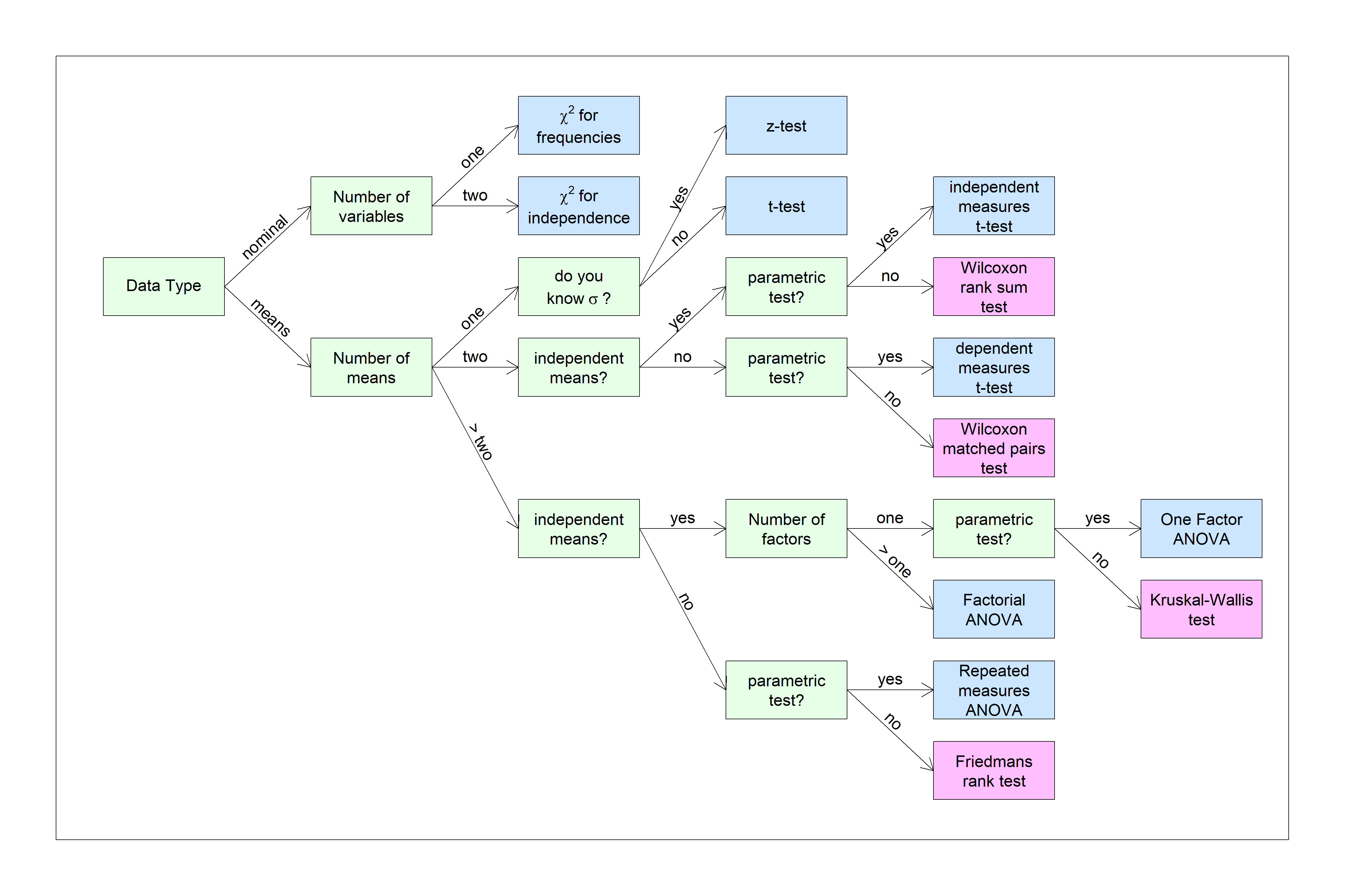
Chapter 25 Tests for Homogeneity of Variance and Normality
There are two assumptions for ANOVA that keep showing up - homogeneity of variance and normality.
Homogeneity of variance is the assumption that each population mean has the same variance - even if \(H_{0}\) is false and the population means are different. Homogeneity of variance is needed so that we can average the variances from each sample to estimate the population variance. The assumption of normality means that the populations that each group is drawn from have normal distributions. Together, these two assumptions assume that for ANOVA, every sample is drawn from a normal distribution with the same population variance, even if the population means aren’t the same.
This chapters covers some of the hypothesis tests for homogeneity of variance and normality. If a test is rejected, then this is evidence that your sample doesn’t satisfy one of the two assumptions. If that’s the case, then you might be advised to run one of the Nonparametric Tests that we cover later.
What if you fail to reject a test for homogeneity of variance or normality? You’ll probably read somewhere that if your data fails to reject one of these tests, then your OK to go on with an ANOVA. But you’re also told that you shouldn’t interpret a null result from a hypothesis test as evidence that \(H_{0}\) is true. And you can really drive yourself crazy if you start thinking about assumptions for the tests to see if you’ve satisfied the assumptions of the ANOVA test. What if you don’t satisfy those assumptions? Is there a test for that? I wish I had something intelligent to say about this.
But a statistics course isn’t complete without covering these tests. So here we go:
25.1 Homogeneity of Variance
The two most common tests for homogeneity of variance are Bartlett’s test and Levene’s test. Of the two, the Levene’s test seems to be by far the most common so we’ll only focus on this one here. Interestingly, Bartlett’s test is more powerful, meaning that it is more likely to detect heterogeneity of variance if it’s there. Could it be that we’re favoring a less powerful test because where we kind of hope that we don’t reject it? After all, if we reject a test for homogeneity of variance, then we’re supposed to run a less powerful nonparametric test on our data. Nobody talks about these things.
25.1.1 Levene’s test (by hand)
The formula for variance starts with calculating the deviation between scores and the mean of the scores. So if your data comes from a population that satisfies homogeneity of variance, then the deviation between each score and the mean of the group that it came from should be, on average, about the same.
This is where Levene’s test starts - with a twist. R’s leveneTest by default first calculates the deviation between each score and the median of the group that it came from. Let’s demonstrate this with some fake data.
First, we define some population parameters - the number of groups (k), the sample sizes (n), and the population means (mu) and standard deviations (sigma). Notice that the first value of sigma is not like the others - we’re violating homogeneity of variance. We should end up rejecting \(H_{0}\) and conclude, correctly, that our population does not have equal variances.
This next step generates a single data set based on these parameters using rnorm to generate vectors x with the associated sample size, mean and standard deviation. The data is organized in long format, holding the (fake) independent variable x, and the corresponding group name (e.g. ‘group 1’).
I’ve also included, for each score, the median for the group that the score came from and a value Z which is the absolute value of the difference between the score and it’s group median abs(x-median(x)):
dat <- as.data.frame(matrix(nrow=0,ncol=3))
for (i in 1:k) {
  x <- round(rnorm(n[i],mu[i],sigma[i]),2)  # this group's sample
  dat <- rbind(dat,data.frame(x,rep(median(x),n[i]),abs(x-median(x)),
                              factor(rep(sprintf('group %d',i),n[i]))))
}
colnames(dat) <- c('x','median','Z','group')
The fake data looks like this:
| x | median | Z | group |
|---|---|---|---|
| 44.94 | 77.35 | 32.41 | group 1 |
| 77.35 | 77.35 | 0.00 | group 1 |
| 36.57 | 77.35 | 40.78 | group 1 |
| 133.81 | 77.35 | 56.46 | group 1 |
| 83.18 | 77.35 | 5.83 | group 1 |
| 61.80 | 74.87 | 13.07 | group 2 |
| 74.87 | 74.87 | 0.00 | group 2 |
| 77.38 | 74.87 | 2.51 | group 2 |
| 75.76 | 74.87 | 0.89 | group 2 |
| 66.95 | 74.87 | 7.92 | group 2 |
| 85.12 | 73.90 | 11.22 | group 3 |
| 73.90 | 73.90 | 0.00 | group 3 |
| 63.79 | 73.90 | 10.11 | group 3 |
| 47.85 | 73.90 | 26.05 | group 3 |
| 81.25 | 73.90 | 7.35 | group 3 |
| 69.55 | 75.94 | 6.39 | group 4 |
| 69.84 | 75.94 | 6.10 | group 4 |
| 79.44 | 75.94 | 3.50 | group 4 |
| 78.21 | 75.94 | 2.27 | group 4 |
| 75.94 | 75.94 | 0.00 | group 4 |
| 79.19 | 76.20 | 2.99 | group 5 |
| 77.82 | 76.20 | 1.62 | group 5 |
| 70.75 | 76.20 | 5.45 | group 5 |
| 50.11 | 76.20 | 26.09 | group 5 |
| 76.20 | 76.20 | 0.00 | group 5 |
You don’t have to follow exactly how the code works. Just understand what each column holds.
If homogeneity of variance is true, then the average value of Z should be about the same for each group. How do we test if the values of Z vary significantly across the groups? ANOVA! Levene’s test is just an ANOVA on Z (Z ~ group):
## Analysis of Variance Table
##
## Response: Z
##           Df Sum Sq Mean Sq F value  Pr(>F)
## group      4 1822.4  455.60  2.8151 0.05288 .
## Residuals 20 3236.8  161.84
## ---
## Signif. codes:  0 '***' 0.001 '**' 0.01 '*' 0.05 '.' 0.1 ' ' 1
25.1.2 Levene’s test (using R)
R’s function for Levene’s test requries the ‘car’ package. Once loaded it works like this:
## Levene's Test for Homogeneity of Variance (center = median)
##       Df F value  Pr(>F)
## group  4  2.8151 0.05288 .
##       20
## ---
## Signif. codes:  0 '***' 0.001 '**' 0.01 '*' 0.05 '.' 0.1 ' ' 1
The numbers match.
25.1.2.1 We actually just ran the Brown-Forsythe test
If you want to impress your friends, because R’s LeveneTest uses the median by default, you can tell them that is actually the Brown-Forsythe test. You can run the true Levene’s test this way:
## Levene's Test for Homogeneity of Variance (center = "mean")
##       Df F value  Pr(>F)
## group  4  3.4503 0.02674 *
##       20
## ---
## Signif. codes:  0 '***' 0.001 '**' 0.01 '*' 0.05 '.' 0.1 ' ' 1
Using the median is apparently more robust to violations of skewness and heavy tails in your sampling distributions. You can learn a little about the difference between using the median vs. mean from Wikipeida’s entry on Levene’s test.
25.1.2.2 Levene’s test on Levene’s test
Want to lose some sleep? Check this out:
## Levene's Test for Homogeneity of Variance (center = median)
##       Df F value  Pr(>F)
## group  4  2.9673 0.04477 *
##       20
## ---
## Signif. codes:  0 '***' 0.001 '**' 0.01 '*' 0.05 '.' 0.1 ' ' 1
What’s this? It’s a test for homogeneity of variance on Z, which is Levene’s test on the ANOVA used for Levene’s test on our original data. For this data set, p<.05, which means that Levene’s test failed its own test for homogeneity. Does this mean we shouldn’t used Levene’s test for this data set? Now what?
25.2 Tests for Normality
There is no single standard test the hypothesis that a sample is drawn from a normal distribution. Instead, there are a variety of tests, each having their own strengths and weaknesses. Here we’ll discuss two of the most common tests, the Lilliefors test and the Shapiro-Wilk test. I chose these two because the first is one of the most common for historical reasons, and the second is considered the most powerful (most likely to correctly detect a deviation from normality).
There are many others, including specific tests for skeweness and/or kurtosis. I found a good pdf on this from NCSS.com that briefly covers a variety of tests. Here’s a link to the pdf which I’ve copied to the course website: http://courses.washington.edu/psy524a/pdf/Normality_Tests.pdf
We’ll use as an example a made-up sample of 50 Grades which can be loaded into R like this:
orig.data<-read.csv("http://www.courses.washington.edu/psy524a/datasets/Grades.csv")
# Pull out the single variable
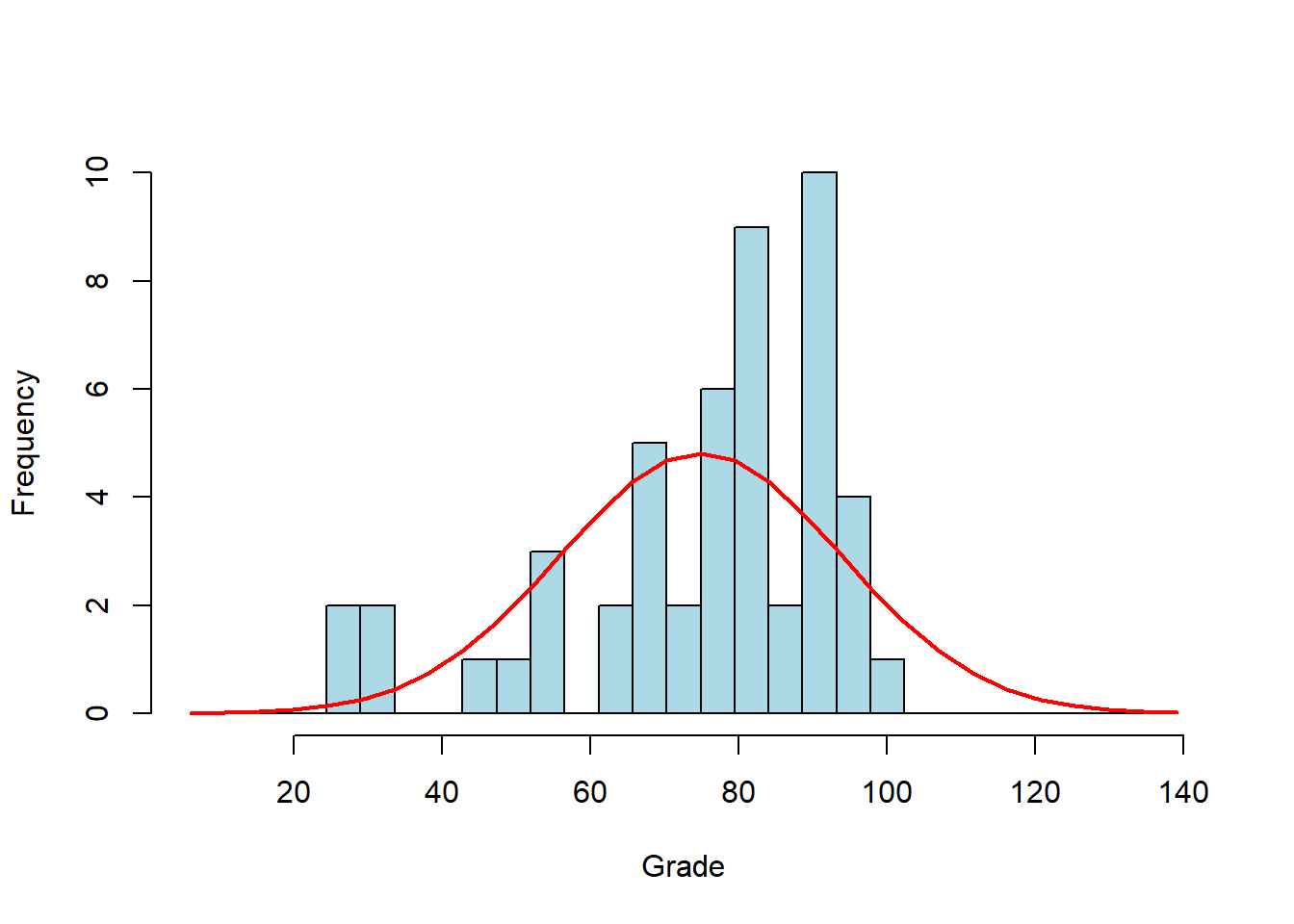
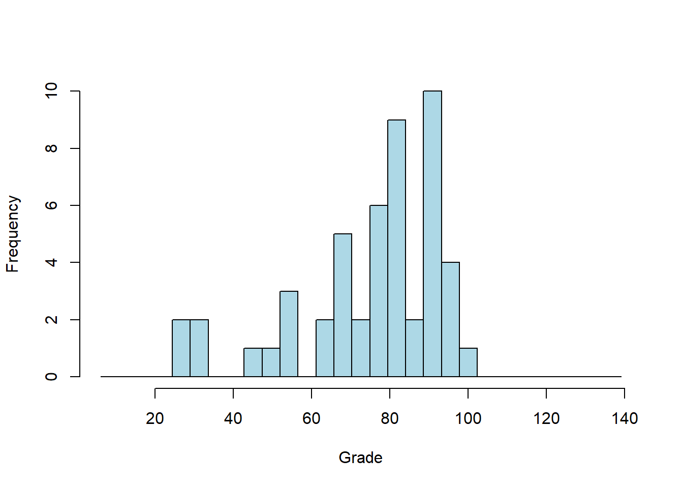
grades <- orig.data$GradeBefore we run any tests for statistical significance, we should first look at the distribution of scores as a histogram. Often simply viewing the shape of the distribution will tell you enough. For this example it looks like our grades don’t seem to be distributed as a familiar bell-shaped curve. Instead, it looks negatively skewed.
All tests for normality compare the distribution of your data to a normal distribution having the same mean and standard deviation of your sample. The actual mean of our scores is 74.9 and the standard deviation is 19. Here is a normal distribution with this mean and standard deviation drawn on top of our histogram:
A common way to compare the distribution of your data to a normal distribution is to compare relative cumulative distributions. As we’ve discussed before (see section 3.6), relative cumulative distributions are the cumulative sum of the histogram as you sweep from left to right, normalized so they sum to 1. Here are the corresponding relative cumulative distributions for the data and the normal curve:
The closer the data points fit the red curve, the closer the data is to normal.
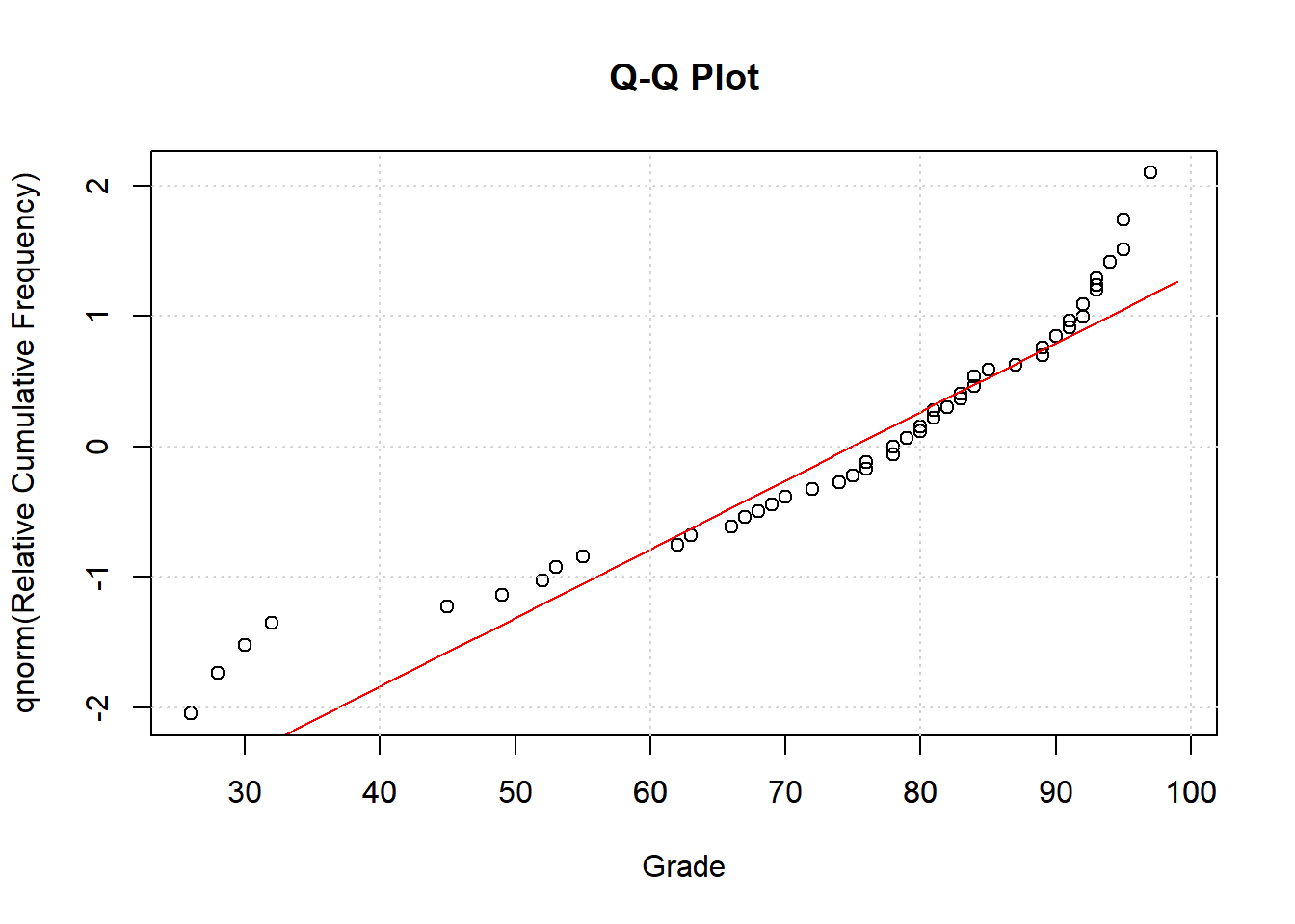
25.2.1 Q-Q Plot
It’s common to convert these cumulative frequency into z-scores by passing them through the inverse of the normal distribution (qnorm in R). This generates what’s called a Q-Q plot, where ‘Q’ stands for ‘quantile’. This transforms the values on the y-axis in the previous plot to z-scores, so that for example a value of .05 becomes -1.6449, 0.5 becomes 0, and .95 becomes 1.6449.
This transformation turns the S-shaped cumulative normal into a straight line, which can be more easily compared to the data:

25.2.2 Lilliefors Test
Formally known as the Kolmogrov-Smirnov test with the Lilliefors correction, this is a hypothesis test on the maximum deviation between the cumulative frequency data and the corresponding curve for the normal distribution.
Lilliefors test is an extension on the Kolmogrov-Smirnov, or KS test which is a test to determine if two distributions came from the same population. However, as a test for normality the KS test is biased because the normal distribution we’re comparing our data to is determined by the mean and standard deviation of our data. So the fit will generally be too good. We really should use the means and standard deviations of the population parameters from the null hypothesis, which we don’t have.
As result, the p-value from the KS test for normality will be too large because a normal distribution based on the sample mean and standard deviation of the data will always be a better fit to the data than one based on the population parameters.
This bias can be fixed with the Lilliefors Significance Correction (the default with SPSS). There is no known formula for this corrected distribution. Tables are based on Monte Carlo simulations.
R has a function called lillie.test in the package nortest. Here’s how to run Lilliefors test on our example data:
lillie.out = lillie.test(grades)
sprintf('Lilliefors test for normality, p = %5.6f',lillie.out$p.value)
## [1] "Lilliefors test for normality, p = 0.010845"According to the Lilliefors test, we should reject the null hypothesis that this sample came from a normal distribution.
25.3 The Shapiro Wilk test
The Lilliefors test has the advantage of simplicity - it’s easy to understand the statistic in terms of the fit of an observed to an expected cumulative frequency. However, it has been criticized as not having sufficient power for detecting violations of normality. Later in this chapter we’ll demonstrate this lack of power.
Instead, some statisticians prefer the Shapiro-Wilk test. The intuition is that the statistic returned from this test, \(W\), is related to the correlation of the data in the Q-Q plot. That is, it can be thought of as a test of how well the Q-Q plot is fit by a straight line. The math behind it isn’t very intuitive, and the statistic \(W\) doesn’t come from one of our parametric friends (e.g. \(\chi^2\), t or F). For a deeper dive, see this reference.
R’s function for the Shapiro Wilk test is called shapiro.test which requires loading the ‘dplyr’ package. Here’s how it works:
shapiro.out <- shapiro.test(grades)
print(sprintf('Shapiro-Wilk test for normality, p = %5.6f',shapiro.out$p.value))
## [1] "Shapiro-Wilk test for normality, p = 0.000138"For this sample of scores the p-value for the Shapiro-Wilk test is way smaller than for the Lilliefors test.
This leads to a dilemma - with such large differences in p-values, which test should you use? After perusing many websites and textbooks, the common thread is that you should eyeball the data via histograms and Q-Q plots. I know that’s not a very satisfying answer. Statisticians seem to be saying that non-normal distributions are like Supreme Court Justice Potter Stewart’s famous 1964 test for obscenity in pornography - “I know it when I see it.”
It turns out that both hypothesis tests led to the correct decision. We know this because I made this data of test scores by drawing 50 values from a \(\chi^{2}\) distribution with three degrees of freedom, multiplying the values by 10 and subtracting it from 100:
100-round(10*rchisq(50,3))
Here’s the actual probability distribution of the population that our sample was drawn from along with the histogram of the sample:
This is not normal.
25.3.1 Power of tests for normality
To my knowledge, there isn’t a function that tests the power for these test for normality. In fact, there isn’t even a measure for effect size. But never fear - we know how to estimate power without a function (or a math education). Simulation!
The following chunk of code generates multiple random samples from the distribution described above (which is not normal). This is done over a range of sample sizes. For each sample, both the Lilliefors test and the Shapiro-Wilk test is run and the p-values are stored:
# Simulate how power increases with sample size
n <- seq(10,100,10) # list of sample sizes
nReps <- 5000 # number of simulations for each sample size
alpha <- .05
# zero out the things
p.lillie <- matrix(data=NA,nrow=length(n),ncol=nReps)
p.shapiro <- matrix(data=NA,nrow=length(n),ncol=nReps)
for (i in 1:length(n)) {
for (j in 1:nReps) {
x <- 100-round(10*rchisq(n[i],3))
# x <- rnorm(n[i]) # use this to test type 1 error rate
lillie.out = lillie.test(x)
p.lillie[i,j] <- lillie.out$p.value
shapiro.out <- shapiro.test(x)
p.shapiro[i,j] <- shapiro.out$p.value
}
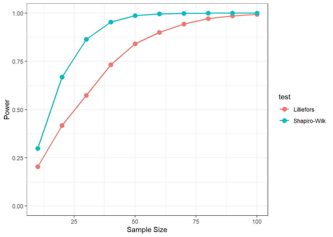
}After the simulation is run, the following chunk plots the proportion of rejected p-values for both tests across the range of sample sizes:
power.lillie <- rowMeans(p.lillie<alpha)
power.shapiro <- rowMeans(p.shapiro<alpha)
dat <- rbind(
  data.frame(n=n,power = power.lillie,test = rep('Lilliefors',length(n))),
  data.frame(n=n,power = power.shapiro,test = rep('Shapiro-Wilk',length(n))))

ggplot(data = dat,aes(x = n,y=power,group = test)) +
  geom_line(aes(color = test),size = .75) +
  geom_point(aes(color = test),size = 3) +
  ylab('Power') +
  ylim(0,1) +
  xlab('Sample Size') +
  theme_bw()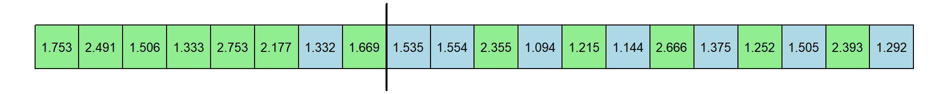
You’ll notice a couple things from this simulation. First, power increases with sample size - which is always the case. Second, the Shapiro-Wilk test has more power than the Liliefors test. This is consistent with our original samle which showed a smaller p-value for the Shapiro-Wilk test than for the LIllliefors test.
If you re-run the analysis with \(H_{0}\) as true (drawing from a normal distribution) you’ll see that the rejection rate hovers around 0.05 for both tests across all sample sizes, which is good.
25.4 Why be normal?
It is a common misconception that your dependent variable in a hypothesis test, like an ANOVA or t-test, needs to be normal to make the test valid. There are two problems with this.
The first is that if we’re running parametric tests on our data, our assumptions require that the means that we’re measuring are coming from a population that is normally distributed. As we all know now, with a large enough sample, the Central Limit Theorem comes to the rescue. So if we’re running a test on means (e.g. t-test or ANOVA) with a sample size of 20 or more, then the assumption of normality for the distributions of means is pretty safe.
Another issue with testing normality on your dependent variable is that what’s actually important is that the residuals after fitting your model to the data are normally distributed.
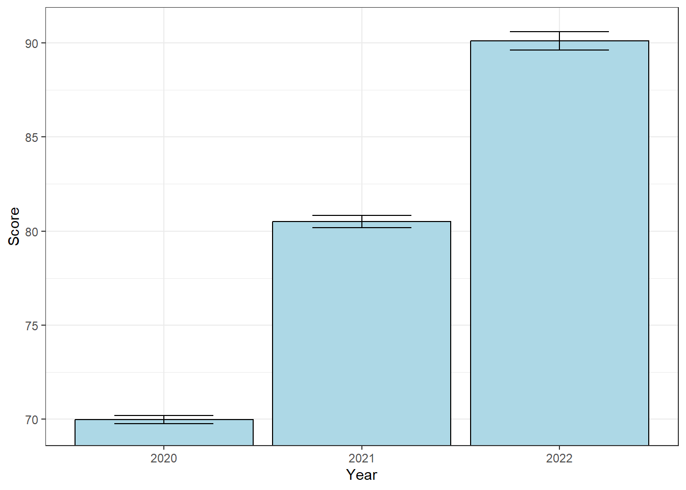
Consider a one-factor fixed-effect ANOVA for exam scores over time. There are 500, 250, and 100 students that took exams in each of the years 2020, 2021, and 2022. Here’s a plot of the means and standard errors:

Consider the overall distribution of our dependent variable, which a histogram of all test scores across all years:
It looks like we’re positively skewed. In fact, a Shapiro-Wilk test gives us a p-value of \(p<0.0001\).
But it shouldn’t be surprising that the distribution of all scores is not normal. The overall distribution of scores is the combination of three separate distributions around the three group means. If the null hypothesis is false, and the means are different, then we would in fact expect a non-normal distribution of our dependent variable.
Instead, what’s important to satisfy the conditions of our hypothesis test is that the residuals are normally distributed. Remember, residuals are the deviations between the model predictions and the data. In the case of ANOVA, the model predictions are the means for each group, so the deviations are the deviations from these means, which are the deviations that contribute to \(SS_w\).
Here’s a histogram of those deviations
The residuals do look normally distributed. Indeed, a Shapiro-Wilk test gives us a p-value of \(p = 0.7949\).