Chapter 20 Correlation and Regression

You’ll often hear the words ‘correlation’ and ‘regression’ in the same context. They are essentially the same thing - both are about the relation between one or more independent variables and a dependent variable. We’ll start with regression by introducing the ‘general linear model’ and apply it to some data from the survey.

20.1 The General Linear Model

A huge part of inferential statistics can be discussed in the framework of ‘The General Linear Model’, or the GLM. You can actually consider just about all inferential statistics in the context of the GLM, including correlations, regression, ANOVA and even $\chi^{2}$ tests. Here we’ll use a specific example to illustrate the relationship between these things.

There are two main assumptions for the GLM. The first is that you can predict a dependent variable as a linear combination of independent variables. A linear combination of a set of numbers is the sum of the numbers after multiplying each by a constant called a weight or coefficient. For now we’ll assume that all variables are continuous, and not categorical. Formally, if $X_{i}$ is your set of independent variables, called regressors, and $\beta_{i}$ is a corresponding set of coefficients, then our dependent variable $Y$ can be predicted as:

\[ \hat{Y} = \beta_0 + \beta_1X_1 + \beta_{2}X_{2} + ... + \beta{k}X_{k} \] Putting a ‘hat’ (‘^’ symbol) on top of a variable means that this a prediction, or estimation, of that variable. So $\hat{Y}$, pronounced ‘Y-hat’, is the GLM’s prediction of the dependent variable, Y.

The difference between the prediction $\hat{Y}$ and the data $Y$ is called the error or residual. A second assumption of the GLM is called homoscedasticity which is that the residuals are distributed normally with mean zero and some standard deviation $\sigma$. We write this as:

\[ Y-\hat{Y} \sim N(0,\sigma) \]

Putting this together, you’ll sometimes see the GLM written as:

\[ Y = \beta_0 + \beta_1X_1 + \beta_{2}X_{2} + ... + \beta{k}X_{k} + N(0,\sigma) \]

20.2 Example: predicting student’s heights from their mother’s heights

Let’s work with a specific example with a single independent variable. With a single independent variable the GLM simplifies to:

\[ Y = \beta_0 + \beta_1X_1 + N(0,\sigma) \] We’ll use survey and try to predict the height of the students that identify as women from their mother’s heights.

survey <-
  read.csv("http://www.courses.washington.edu/psy315/datasets/Psych315W21survey.csv")

id <- survey$gender== "Woman" & 
  !is.na(survey$height) & !is.na(survey$mheight) &!is.na(survey$pheight) &
  survey$mheight > 55  &  # remove outliers
  survey$height > 55

X <- survey$mheight[id]
Y <- survey$height[id]
Z <- survey$pheight[id]  # save fathers heights for later
heights <- data.frame(student = Y, mother = X, father = Z)

It helps to visualize the data as a scatterplot:

n <- length(X)
p <- ggplot(heights, aes(x=X, y=Y)) + 
  geom_point(shape = 21,size= 3) +
  geom_point(shape = 21,size= 3,fill = "green",alpha = .075) + theme_bw() +
  xlab('Mother\'s height (in)') + ylab('Student\'s height (in)')
plot(p)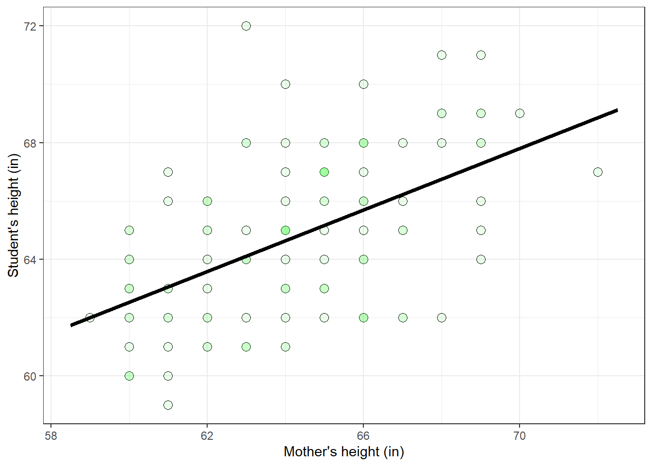

There is a clear tendency for taller mothers to have taller daughters.

If we let $X$ be the mother’s height and $Y$ be the student’s height, then the GLM predicts that:

\[ \hat{Y} = \beta_0 + \beta_1X \] The GLM predicts a straight line through the scatterplot with a slope $\beta_1$ and intercept $\beta_0$.

What does it mean by ‘fit the data’? For fitting the GLM, we define the goodness of fit as the sums of squares of the residuals:

\[ SS_{YX} = \sum(Y-\hat{Y})^{2} \]

Warning: this chapter has a lot of similar looking symbols and formulas. See the glossary at the end of this chapter for reference.

We need to find the values of $\beta_0$ and $\beta_1$ that make $SS_{YX}$ as small as possible.

A quick note about squaring - statisticians love squaring things. There are good reasons for this - it’s an easy way to make things positive, and squaring has nice properties like having a continuous second derivative, and it’s relationship to the mean. Squaring makes finding the best fitting parameters computationally easy and robust.

20.3 Regression

Finding the best-fitting coefficients for the GLM is called regression.

For a single independent variable, there is a closed-form solution. If we first calculate the mean of X ($\overline{X}$) and the mean of Y ($\overline{Y}$), then:

\[ \beta_1 = \frac{\sum{(X-\overline{X})(Y-\overline{Y})}}{\sum{(X-\overline{X})^2}} \] and

\[ \beta_0 = \overline{Y} - \beta_1\overline{X} \] The $\Sigma$ means to sum across all data points. With R, we can calculate these coefficients like this:

beta_1 <- sum((X-mean(X))*(Y-mean(Y)))/sum((X-mean(X))^2)
beta_0 <- mean(Y) - beta_1*mean(X)
beta_0

## [1] 30.78893

beta_1

## [1] 0.5288607

So (rounding to 2 decimal places) the best fitting line through the scatterplot is:

\[ \hat{Y} = 30.79 + 0.53X \] This line is called the regression line. Here’s the regression line drawn over the scatterplot of the data:

xplot <- c(min(X)-.5,max(X)+.5)
yplot <- beta_0 + beta_1*xplot
regression_data <- data.frame(x=xplot,y=yplot)
p_regression_line <- geom_line(data = regression_data,aes(x=x,y=y), linewidth = 1.5 )
p + p_regression_line

The sums of squares of the residuals, called $SS_{YX}$, can be calculated like this:

Y_hat <- beta_0 + beta_1*X
SS_YX <- sum((Y-Y_hat)^2)
SS_YX

## [1] 659.1687

No matter how hard you try, you’ll never find a better pair of coefficients ($\beta_0$ = 30.79, $\beta_1$ = 0.53) that will produce a sums of squared error less than $SS_{YX}$ = 659.1687

20.4 Regression using ‘lm’

R has a very flexible function, lm, for calculating best-fitting regression coefficients. You’ve already used it in our previous chapters on ANOVA. It works by defining a ‘model’ based on the independent and dependent variables in your data frame. For our example, we write the model predicting student’s heights (Y) from mother’s heights (X) simply as $Y \sim X$. The result is an object that contains the best-fitting coefficients along with a lot of other stuff.

lm.out <- lm(student ~ mother, data = heights)
lm.out$coefficients

## (Intercept)      mother 
##  30.7889348   0.5288607

There are our values of $\beta_0$ and $\beta_1$.

The residuals for every data point are in the field $residuals, so $SS_{YX}$ can be calculated as:

sum(lm.out$residuals^2)

## [1] 659.1687

20.5 Residuals

Remember, the second part of the GLM is that the residuals ($Y-\hat{Y}$) are distributed normally. Here’s a plot of the residuals:

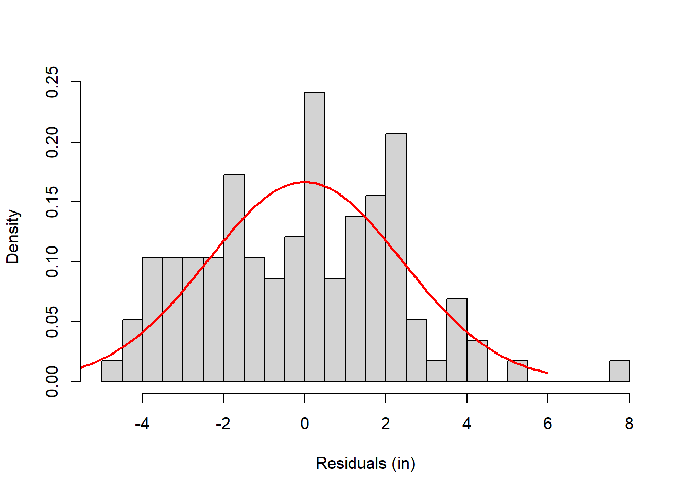
hist(Y-Y_hat,breaks = 20,xlab = 'Residuals (in)',main = NULL)

It’s not perfect - but it never is. Later on we’ll cover the chapter on test for normality Tests for Homogeneity of Variance and Normality that covers how to run a The Shapiro Wilk test or Lilliefors Test test for normality. The Shapiro Wilk tests for normality results in a p-value of p=0.094, which means we fail to reject the null hypothesis that this sample was drawn from a normal distribution. In other words, the residuals are normal enough.

20.6 The standard error of the estimate, $S_{YX}$

Since the residuals are the error left over after fitting the model, the standard deviation of these residuals is an estimate of the standard deviation of $\sigma$, the ‘error’ at the end of the GLM equation. This is why the standard deviation of the residuals is called the standard error of the estimate, and gets its own symbol $S_{YX}$. Using the formula for the sample standard deviation:

\[ S_{YX} = \sqrt{\frac{\sum{(Y-\hat{Y})^{2}}}{n-1}} \] You should recognize the formula for the sums of squares of the residuals in there $SS_{Y} = \sum(Y-\overline{Y})^{2}$, so equivalently:

\[ S_{YX} = \sqrt{\frac{SS_{YX}}{n-1}} \] The standard error of the estimate, $S_{YX}$ is 2.4 inches for our example. Here’s that same histogram drawn with a normal distribution centered at zero and standard deviation of 2.4 inches.

S_YX <- sd(Y-Y_hat)
hist(Y-Y_hat,prob = T,breaks = 20,xlab = 'Residuals (in)',main = NULL)
xnorm <- seq(-2.5*S_YX,2.5*S_YX,length = 101)
ynorm <- dnorm(xnorm,0,S_YX)
lines(xnorm,ynorm, col = "red", lwd = 2)

20.6.1 homoscedasticity

Another assumption that we need for regression is ‘homoscedasticity’, which means that not only are the residuals normally distributed, but also the variance of the distribution does not change with the dependent variable. Graphically, homoscedasticity means that the scatter above and below the regression line normally distributed with a constant standard deviation as you slide along the independent variable (the X-axis).

Here’s the scatterplot a shaded region that covers $\pm$ one $S_{YX}$, or 2.4 inches above and below the regression line.

plot_poly <- data.frame(x = regression_data$x[c(1,2,2,1)], 
                        y = regression_data$y[c(1,2,2,1)]+ c(S_YX,S_YX,-S_YX,-S_YX))

p +  p_regression_line  +
  geom_polygon(data = plot_poly,aes(x=x,y=y),fill = "blue",alpha = .4)

For a normal distribution, about 68% of the data points should fall within $\pm$ one standard deviation from the mean. With homoscedasticity, about 68% of the data points should fall within the shaded region in the plot above. It turns out that for this data set, about 85% of the data falls within $\pm$ 2.4 inches of the regression line. Not perfect, but pretty close.

20.7 Correlation

The strength of the relation between the student’s and mother’s heights can be quantified with Pearson product-moment correlation coefficient, sensibly referred to as just correlation. Though there are other measures of correlation, the Pearson correlation is really the default. The correlation, which ranges between -1 and 1, reflects how well the regression line fits the data. A correlation of -1 means that all the data points fall exactly on a downward sloping regression line, and a correlation of 1 means that all the points fall exactly on an upward sloping regression line. Values in between mean that there’s some scatter around the regression line.

The correlation is calculated as:

\[ r = \frac{\sum{(X-\overline{X})(Y-\overline{Y})}}{\sqrt{\sum{(X-\overline{X})^{2}}\sum{(Y-\overline{Y})^{2}}}}\] R has the ‘cor’ function for this:

r <- cor(X,Y)
r

## [1] 0.5217662

Just to show that ‘cor’ isn’t doing something mysterious, here’s how to do it by hand in R:

sum((X-mean(X))*(Y-mean(Y)))/sqrt(sum((X-mean(X))^2)*sum((Y-mean(Y))^2))

## [1] 0.5217662

20.8 The relationship between r and the slope, $\beta_1$

There’s a simple relationship between the correlation, $r$, and the slope of the regression line, $\beta_1$:

\[ \beta_1 = r\frac{S_{Y}}{S_{X}} \] Where $S_{Y}$ and $S_{X}$ are the standard deviations of X and Y. Scaling the X or Y variable will affect the slope of the regression line, $\beta_1$. For example, converting the student’s heights from inches to feet (dividing by 12) will divide the slope of the regression line by 12. But this conversion does not affect the correlation, $r$. In the formula above, see how dividing Y by 12 will divide $S_{Y}$ by 12 which will then divide the slope, $\beta_1$ by 12.

20.9 The relationship between $r^{2}$ and $S_{YX}$

You can think of the residuals in the GLM as the variability in the dependent variable that you can’t explain by the dependent variables. We therefore call the variance of the residuals, which is the square of the standard error of the estimate: $S^{2}_{YX}$, the variance in Y not explained by X. If $S^{2}_{YX}$ is small, then the regression line fits the data well and there’s not much variance left over to ‘explain’. But what does ‘small’ mean? A good measure is the ratio of $S^{2}_{YX}$ to the variance in Y alone, $S^{2}_{Y}$. This ratio has a special relationship to the correlation:

\[ 1-r^{2} = \frac{S^{2}_{YX}}{S^{2}_{Y}} \] In words, $1-r^{2}$ is the proportion of the total variance in Y not explained by X. Turning things around a bit we get:

\[ r^{2} = 1-\frac{S^{2}_{YX}}{S^{2}_{Y}} \] Which means that the square of the correlation, $r^{2}$, is the proportion of variance in Y explained by X and is a commonly reported number. If we have a ‘perfect’ correlation of $r=1$ or $r=-1$, then $r^{2}=1$, and all of the variance in Y is explained by X. If there is no correlation ($r=0$) then none of the variance in Y is explained by X.

We can verify the relationship between the correlation $S^{2}_{YX}$ and $S^{2}_{Y}$ with our example in R:

1-S_YX^2/var(Y)

## [1] 0.2722399

r^2

## [1] 0.2722399

For our example, about 27% of the variance in the student’s heights can be explained by their mother’s heights. The remaining 73% of the variance in the student’s heights must be due to other factors (like their father’s heights, random genetic factors, etc.)

20.10 Statistical significance of regression coefficients

Great, so we know that there is a positive regression coefficient, $\beta_1 = 0.53$ that describes how student’s heights increase with their mother’s heights. But do we really need this regressor to improve the fit? Specifically, does including mother’s heights as a factor significantly improve the fit compared to a simpler model? The simpler model, called the ‘null’ model contains only the intercept:

\[ Y = \beta_0 + N(0,\sigma) \] The best-fitting value of $\beta_0$ is the number that minimizes the sums of squared deviations from that value. Remember what that value is? It’s the mean! $\overline{Y}$ It’s a silly model - it says that no matter what X is, our best guess of Y is the mean of Y. The sums of squares of the the residuals for the null model is $\sum{(Y-\overline{Y})^2}$, which is $SS_{Y}$. To specify the null model using lm in R we use Y ~ 1:

lm_null.out <- lm(Y ~ 1, data = heights)
lm_null.out$coefficients

## (Intercept) 
##       64.75

This value is the mean of Y:

mean(Y)

## [1] 64.75

The sums of squares of the residuals is:

SS_Y <- sum((Y-mean(Y))^2)
SS_Y

## [1] 905.75

Which is the same as

sum(lm_null.out$residuals^2)

## [1] 905.75

By adding $\beta_1X$ to the model, our sums of squared error went down from $SS_{Y}$ =905.75 to $SS_{YX}$ = 659.17, a difference of 246.58.

The model Y ~ X and Y ~ 1 are called nested because one is a simpler version of another. It is implied that the model Y ~ X is really Y ~ 1 + X (try it in R, you’ll get the same thing). Two models are nested if one shares a subset of the regressors than the other.

We call the more complicated model the complete model and the null model the restricted model. Adding a regressor to a model will always improve the fit because one option for the new model is to have the coefficient equal to zero, which is the same as the restricted model.

You can run a hypothesis test to see if the complete model has a significantly smaller SS than the null model using a nested F test, where:

\[ F = \frac{(SS_{r}-SS_{c})/(k_{c}-k_{r})}{SS_{c}/(n-k_{c})} \] $SS_{r}$ and $SS_{c}$ are the sums of squares errors for the restricted and complete models, $k_{r}$ and $k_{c}$ are the number of regressors for the two models, and $n$ is the total number of data points. The F statistic has $k_{c}-k_{r}$ degrees of freedom in the numerator, and $n-k_{c}$ degrees of freedom in the denominator.

For our example, there are two regressors, $\beta_0$ and $\beta_1$ for the complete model, so $k_{c} = 2$, and one regressor for the restricted model, so $k_{r}$ = 1. There are $n=116$ data points, so:

\[ F = \frac{(SS_{Y}-SS_{YX})/(2-1)}{SS_{YX}/(n-2)} = \frac{(905.75 -659.17)/1}{659.17/(116-2)} = 42.65 \]

The degrees of freedom are 1 and n-2 = 114. The p-value can be found using the pf function in R:

pf_value <- 1-pf(F_stat,1,n-2)
print(sprintf('F(%d,%d) = %5.3f, p = %g',1,n-2,F_stat,pf_value))

## [1] "F(1,114) = 42.645, p = 1.9006e-09"

This is a teeny tiny p-value, which means that adding the mother’s height as a regressor significantly improves the prediction of the student’s height.

This was just to show you how to do this by hand. R runs the same analysis by passing the output of lm into the anova function, like we did for ANOVA’s in the previous chapters:

anova(lm.out)

## Analysis of Variance Table
## 
## Response: student
##            Df Sum Sq Mean Sq F value    Pr(>F)    
## mother      1 246.58 246.581  42.645 1.901e-09 ***
## Residuals 114 659.17   5.782                      
## ---
## Signif. codes:  0 '***' 0.001 '**' 0.01 '*' 0.05 '.' 0.1 ' ' 1

Without telling you, ‘lm’ ran the null model on its own and did its own nested F test. You should recognize most of these numbers. The first column are the two degrees of freedom. The second column are sums of squares. The bottom row is the residual sums of squares for the complete model, $S_{YX}= 659.17$. The sums of squares for the row labeled ‘X’ is the difference in sums of squares between the complete and the restricted model, which we calculated before:

\[SS_{Y}-SS_{YX} = 905.75 - 659.17 = 246.58\]

The column labeled ‘Mean Sq’ is the sums of squares for each row divided by their degrees of freedom. And there’s our F statistic and corresponding p-value.

20.11 Statistical significance of correlations

Another hypothesis test whether or not the correlation is significantly different from zero. The null hypothesis that there is no correlation in the population that you’re drawing from. Formally, the parameter, $\rho$, is the correlation in the population and the null hypothesis is that $\rho = 0$.

Sir Ronald Fisher worked out that the distribution of correlations drawn from a population with zero correlation can be approximated by a t-distribution using the formula:

\[ t = \frac{r}{\sqrt{\frac{1-r^{2}}{n-2}}} \]

with $df = n-2$. For our example, using R, we can use pf to get a p-value:

n <- length(X)
t <- r/sqrt((1-r^2)/(n-2))
pt_value <- 2*(1-pt(t,n-2)) # 2* for a two-tailed test
print(sprintf('t(%d) = %5.4f, p = %g',n-2,t,pt_value))

## [1] "t(114) = 6.5303, p = 1.9006e-09"

R has it’s own function, cor.test for this:

out.cor <- cor.test(X,Y)
out.cor

## 
##  Pearson's product-moment correlation
## 
## data:  X and Y
## t = 6.5303, df = 114, p-value = 1.901e-09
## alternative hypothesis: true correlation is not equal to 0
## 95 percent confidence interval:
##  0.3751349 0.6429236
## sample estimates:
##       cor 
## 0.5217662

You should see some familiar numbers there.

Compare this p-value to the nested F-test above. They’re exactly the same! We’ve just demonstrated that these two hypotheses tests are identical. Notice, also, that if you square the t-statistic from the correlation test you get the F statistic from the nested F test: $6.53^{2} = 42.645$. Recall that for an ANOVA with two levels, we also found that $t = F^2$.

20.12 Why two identical hypothesis tests?

We’ve covered two ways of testing the statistical significance of the effect of mother’s heights on student’s heights. The first was the t-test on the correlation and the second was an F-test on the sums of squared errors.

Why do we have two tests that get the same answer? It’s probably because they look at the problem from different perspectives. The t-test on correlations is about testing if the relation between X and Y is significantly strong, and the F-test is about whether adding X to the null model significantly improves the goodness of fit. At least they get the same answer.

20.13 Glossary of terms

	description	formula
$SS_{Y}$	Sums of squared deviation from the mean	$\sum{(Y-\overline{Y})^{2}}$
${S^{2}}_{Y}$	Variance of Y	$\frac{SS_{Y}}{n-1}$
$S_{Y}$	Standard deviation of Y	$\sqrt{{S^{2}}_{Y}}$
$\hat{Y}$	Predicted value of Y	$\hat{Y} = \beta_0+\beta_1{X}$
$SS_{YX}$	Sums of squared residuals	$\sum{(Y-\hat{Y}})^{2}$
${S^{2}}_{YX}$	Variance of Y not explained by X	$\frac{SS_{YX}}{n-1}$
$S_{YX}$	standard error of the estimate	$\sqrt{{S^{2}}_{YX}}$

	description	formula
\(SS_{Y}\)	Sums of squared deviation from the mean	\(\sum{(Y-\overline{Y})^{2}}\)
\({S^{2}}_{Y}\)	Variance of Y	\(\frac{SS_{Y}}{n-1}\)
\(S_{Y}\)	Standard deviation of Y	\(\sqrt{{S^{2}}_{Y}}\)
\(\hat{Y}\)	Predicted value of Y	\(\hat{Y} = \beta_0+\beta_1{X}\)
\(SS_{YX}\)	Sums of squared residuals	\(\sum{(Y-\hat{Y}})^{2}\)
\({S^{2}}_{YX}\)	Variance of Y not explained by X	\(\frac{SS_{YX}}{n-1}\)
\(S_{YX}\)	standard error of the estimate	\(\sqrt{{S^{2}}_{YX}}\)

Introduction to Statistics and Data Analysis