Chapter 24 Logistic Regression
Logistic regression is just like regular linear regression (and therefore like ANOVA) except that the dependent variable is binary - zeros and ones. Here we’ll work with a specific example from research with Ione Fine and grad student Ezgi Yucel. Ezgi obtained behavioral data from patients with blindness that had received retinal implants. These patients, who had lost sight due to retinal disease, had an array of stimulating electrodes implanted on their retinas (Argus II, Second Sight inc.) When current is pulsed through these electrodes some of the remaining retinal cells are stimulated, leading to a visual percept.
Ideally, each electrode should lead to a single percept, like a spot of light. A desired image could then be generated by stimulating specific patterns of electrodes. But sometimes it doesn’t work out this way. Simultaneously stimulating some pairs of electrodes leads to a single percept. The percepts induced by single electrodes are large enough that simulating neighboring electrodes can lead to a single ‘blob’. Also, the size of the percept increases with the amplitude of the current, so high currents can also cause percepts to merge. The ability to see two separate spots therefore depends on how far the electrodes are physically far apart and the amplitude of the current.
24.1 Example data: visual percepts for retinal prostheses patients
Ezgi stimulated various pairs of electrodes simultaneously at a range of amplitudes and asked three patients to choose whether they saw one or two percepts. The data is loaded in from the csv file here:
Here’s what the data structure looks like:
| amp | dist | resp |
|---|---|---|
| 331 | 1818.3097 | 0 |
| 299 | 2370.7857 | 0 |
| 565 | 3352.7973 | 1 |
| 387 | 2875.0000 | 1 |
| 387 | 2875.0000 | 1 |
| 452 | 2073.1920 | 1 |
| 299 | 2370.7857 | 1 |
| 412 | 3450.0000 | 1 |
| 266 | 2300.0000 | 1 |
| 533 | 1285.7391 | 0 |
| 266 | 2300.0000 | 0 |
| 387 | 2875.0000 | 1 |
| 500 | 4146.3840 | 1 |
| 266 | 2300.0000 | 1 |
| 419 | 813.1728 | 0 |
| 419 | 813.1728 | 0 |
| 299 | 2370.7857 | 1 |
| 533 | 1285.7391 | 0 |
| 565 | 3352.7973 | 1 |
| 419 | 813.1728 | 0 |
| 331 | 1818.3097 | 0 |
| 412 | 3450.0000 | 1 |
| 412 | 3450.0000 | 1 |
| 533 | 1285.7391 | 0 |
| 565 | 3352.7973 | 1 |
| 500 | 4146.3840 | 1 |
| 452 | 2073.1920 | 1 |
| 331 | 1818.3097 | 0 |
| 500 | 4146.3840 | 1 |
| 452 | 2073.1920 | 1 |
| 484 | 2073.1920 | 1 |
| 460 | 1818.3097 | 1 |
| 379 | 1818.3097 | 0 |
| 435 | 2571.4782 | 1 |
| 379 | 1818.3097 | 0 |
| 484 | 2073.1920 | 1 |
| 395 | 2073.1920 | 1 |
| 435 | 2571.4782 | 1 |
| 395 | 2073.1920 | 1 |
| 435 | 2571.4782 | 1 |
| 460 | 1818.3097 | 1 |
| 420 | 575.0000 | 1 |
| 484 | 2073.1920 | 1 |
| 444 | 1150.0000 | 0 |
| 379 | 1818.3097 | 1 |
| 420 | 575.0000 | 0 |
| 420 | 575.0000 | 0 |
| 428 | 1285.7391 | 1 |
| 444 | 1150.0000 | 0 |
| 428 | 1285.7391 | 0 |
| 476 | 1285.7391 | 1 |
| 460 | 1818.3097 | 1 |
| 476 | 1285.7391 | 1 |
| 395 | 2073.1920 | 0 |
| 403 | 3096.4698 | 1 |
| 444 | 1150.0000 | 0 |
| 476 | 1285.7391 | 1 |
| 403 | 3096.4698 | 1 |
| 428 | 1285.7391 | 0 |
| 403 | 3096.4698 | 1 |
| 270 | 575.0000 | 0 |
| 427 | 813.1728 | 0 |
| 540 | 1725.0000 | 0 |
| 379 | 2370.7857 | 1 |
| 383 | 2571.4782 | 0 |
| 427 | 1818.3097 | 0 |
| 343 | 1285.7391 | 0 |
| 452 | 3096.4698 | 1 |
| 540 | 2073.1920 | 0 |
| 540 | 1725.0000 | 0 |
| 452 | 3681.7964 | 1 |
| 383 | 2571.4782 | 0 |
| 343 | 1285.7391 | 1 |
| 343 | 1285.7391 | 0 |
| 343 | 2370.7857 | 1 |
| 427 | 813.1728 | 0 |
| 492 | 2571.4782 | 1 |
| 270 | 575.0000 | 0 |
| 500 | 1150.0000 | 1 |
| 500 | 1150.0000 | 0 |
| 540 | 1725.0000 | 1 |
| 270 | 575.0000 | 0 |
| 427 | 1818.3097 | 0 |
| 540 | 2073.1920 | 1 |
| 427 | 1818.3097 | 0 |
| 452 | 3681.7964 | 1 |
| 492 | 2571.4782 | 1 |
| 467 | 2073.1920 | 1 |
| 343 | 2370.7857 | 1 |
| 492 | 2571.4782 | 1 |
| 379 | 2370.7857 | 1 |
| 427 | 813.1728 | 0 |
| 540 | 2073.1920 | 1 |
| 452 | 3096.4698 | 1 |
| 467 | 2073.1920 | 1 |
| 295 | 2300.0000 | 1 |
| 295 | 2300.0000 | 1 |
| 343 | 2370.7857 | 1 |
| 295 | 2300.0000 | 1 |
| 452 | 3096.4698 | 1 |
| 467 | 2073.1920 | 1 |
| 452 | 3681.7964 | 1 |
| 379 | 2370.7857 | 1 |
| 500 | 1150.0000 | 1 |
| 383 | 2571.4782 | 1 |
Each row is a trial. We’ll focus on two independent variables:
amp: the amplitude of the current
dist: the distance between the pairs of electrodes (\(\mu m\))
and the dependent variable:
resp: whether the patient saw one percept (resp=0) or two percepts (resp=1)
We’ll be studying the effect of distance on the patient’s reported percepts.
The easiest way to plot the data is to place distance on the x-axis and the patient’s response on the y-axis. Remember, 0 is for trials when they saw one percept and 1 is when they saw two percepts.
p <- ggplot(myData, aes(x=dist, y=resp)) +
  scale_y_continuous(breaks = seq(0,1,by = 0.2)) +
  scale_x_continuous(breaks = seq(0,5000, by = 500)) +
  labs(x = 'Electrode Separation (um)',y='P(two percepts)') +
  theme_bw()
p + geom_point(shape =21, size = 3, fill = 'red') 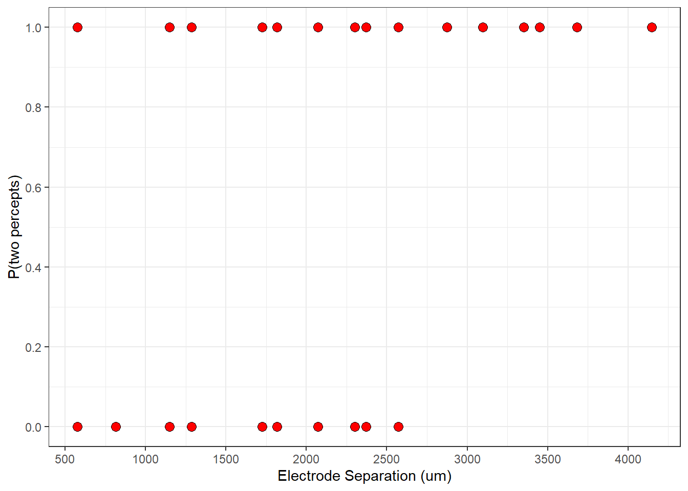
Since the response is binary, it’s hard to see what’s going on here, but you can probably tell that there are more ‘1’ responses at larger distances.
A better way to visualize binary data is to bin the distances into class intervals and take the average number of 1’s in each bin. Here’s one way to do this using a for loop:
# define the bin boundaries
nBins <- 10
bins <- seq(min(myData$dist),
            max(myData$dist)+1,
            length.out = nBins+1)
# zero out the vectors to be filled in the loop
Presp <- numeric(nBins)
nresp <- numeric(nBins)
for (i in 1:nBins) {
  id <- myData$dist >= bins[i] & myData$dist < bins[i+1]
  nresp[i] <- sum(id)
  Presp[i] <- mean(myData$resp[id])
}
binCenter = (bins[1:nBins]+bins[2:(nBins+1)])/2
binned_data <- data.frame(distance = binCenter,Presp)
p <- p+ geom_point(aes(x=distance,y=Presp),data = binned_data, shape = 21,size= (nresp)/5+2,fill = "red")
plot(p)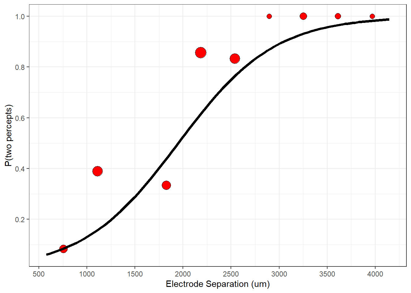
Now you can see a clear effect of distance on the percept. Electrodes that are farther apart from each other have a higher probability of producing two percepts. I’ve scaled the size of the points to represent the number of trials that fall into each bin. Some bins may have no data, which is why you might see a ‘missing values’ warning from ggplot if you run this yourself.
If this were linear regression, we could study the effect of distance on the responses using ‘lm’ like this:
lm(resp ~ dist , data = myData)
This would fit a straight line through the data. This is clearly not appropriate. For one thing, the linear prediction can go below zero and above 1, and that’s not right. But be careful - R will let you run linear regression on a binary dependent variable, and the results might look sensible.
Notice how the data points rise up in a sort of S-shaped fashion. Logistic regression is essentially fitting an S-shaped function to the binary data and running a hypothesis test on the best-fitting parameters.
Logistic regression differs from linear regression in two ways. The first difference is that while linear regression fits data with straight lines, logistic regression uses a specific parameterized S-shaped function called the ‘logistic function’ which ranges between zero and one. The second difference is the ‘cost function’. While linear regression uses sums-of-squared error as a measure of goodness of fit, logistic regression uses a cost function called ‘log-likelihood’.
24.2 The logistic function
To predict the probability of a ‘1’, the model first assumes a linear function of the independent variable (or variables), just like for linear regression. For a single factor:
\[ y = \beta_{0} + \beta_{1}x \]
x is the independent variable, which is distance in our example, and \(\beta_{0}\) and \(\beta_{1}\) are free parameters that will vary to fit the data.
The result, y, is then passed through the S-shaped logistic function which produces the predicted probability that the dependent variable is a ‘1’.
\[ p = \frac{1}{1+e^{-y}} \]
Notice that these two parameters \(\beta_{0}\) and \(\beta_{1}\) are a lot like the intercept and slope in linear regression. They have similar interpretations for logistic regression.
Why do we use the logistic function? There are actually many parameterized S-shaped functions that would probably work just as well, such as the cumulative normal and the Weibul function.
24.3 logistic function parameters: the odds ratio and log odds ratio
One good reason is that the logistic function has special meaning in terms of the ‘log odds ratio’.
If p is the probability of getting a ‘1’, then (1-p) is the probability of getting a ‘0’. The odds ratio is the ratio of the two:
\[ \frac{p}{1-p} \] The log odds ratio is the log of the odds ratio (duh)
\[ log(\frac{p}{1-p}) \]
The odds ratio of getting heads on an unbiased coin flip is 1. The odds of rolling a 1 on a six sided die is 1/5 (sometimes read as ‘one to five’).
With a little algebra, you can show that the formula above can be worked around so that:
\[ y = \beta_{0} + \beta_{1}x = log(\frac{p}{1-p}) \]
In words, logistic regression is like linear regression after converting your data into a log odds ratio.
The parameter \(\beta_{0}\) predicts the log odds ratio when \(x=0\). For our data, patients should always see one percept when the distance is zero. If we assume that the probability of reporting two percepts is 2% with zero distance, then \(\beta_{0} = log(\frac{0.02}{1-0.02}) = -3.9\)
The parameter \(\beta_{1}\) determines how much the log odds ratio increases with each unit increase in x. Positive values of \(\beta_{1}\) predict higher probabilities of ‘1’ with increasing x (like our data). Negative values of \(\beta_{1}\) predict that the probability of a 1 decreases with x. We’ll start with a value of \(\beta_{1} = 0.002\).
Here is a plot of the binned data with the smooth parametrized logistic function:
beta_0 <- -3.9
beta_1 <- 0.002
nPlot <- 101
# x-axis values
xPlot <- seq(min(myData$dist),
             max(myData$dist),
            (max(myData$dist)-min(myData$dist))/nPlot)
# logistic function
y<- beta_0 + beta_1*xPlot
yPlot <- 1/(1+exp(-y))
plot_data <- data.frame(x = xPlot,y=yPlot)
p + geom_line(data = plot_data,aes(x=x,y=y), linewidth = 1.5 )
This seems like a good start, but probably not the best prediction. Logistic regression is all about finding the best parameters that predict the data. What does ‘best’ mean? We need to define a measure of goodness of fit - called a ‘cost function’ and then find the parameters that minimize it.
24.4 The log-likelihood cost function
For linear regression the cost function is the sum if squares of the deviation between the data and the predictions. But a least squares fit is not appropriate for binary data, even if we have an S-shaped prediction. Instead, we’ll define a new cost function called ‘log-likelihood’.
‘likelihood’ and probability are often used interchangeably, but they’re not quite the same thing. Probability is the proportion of times an event will occur. In our example, the logistic function predicts the probability that a patient will report ‘2’ as a function of the distance between electrodes. In this context, probability about predicting the binary dependent variable as we vary the independent variable.
Likelihood is about how well the data is predicted as we vary the model parameters. Likelihood is also a probability - it’s the probability that you’ll obtain a given data set given a specific model.
Here’s how the likelihood of obtaining our data is calculated from the parameters \(\beta_{0} = -3.9\) and \(\beta_{1} = 0.002\).
Consider the first few trials in our experiment:
| dist | resp | predicted |
|---|---|---|
| 1818.3097 | 0 | 0.4345 |
| 2370.7857 | 0 | 0.6988 |
| 3352.7973 | 1 | 0.9430 |
| 2875.0000 | 1 | 0.8641 |
| 2875.0000 | 1 | 0.8641 |
| 2073.1920 | 1 | 0.5613 |
| 2370.7857 | 1 | 0.6988 |
| 3450.0000 | 1 | 0.9526 |
| 2300.0000 | 1 | 0.6682 |
| 1285.7391 | 0 | 0.2094 |
| 2300.0000 | 0 | 0.6682 |
| 2875.0000 | 1 | 0.8641 |
| 4146.3840 | 1 | 0.9878 |
| 2300.0000 | 1 | 0.6682 |
| 813.1728 | 0 | 0.0933 |
| 813.1728 | 0 | 0.0933 |
| 2370.7857 | 1 | 0.6988 |
| 1285.7391 | 0 | 0.2094 |
| 3352.7973 | 1 | 0.9430 |
| 813.1728 | 0 | 0.0933 |
| 1818.3097 | 0 | 0.4345 |
| 3450.0000 | 1 | 0.9526 |
| 3450.0000 | 1 | 0.9526 |
| 1285.7391 | 0 | 0.2094 |
| 3352.7973 | 1 | 0.9430 |
| 4146.3840 | 1 | 0.9878 |
| 2073.1920 | 1 | 0.5613 |
| 1818.3097 | 0 | 0.4345 |
| 4146.3840 | 1 | 0.9878 |
| 2073.1920 | 1 | 0.5613 |
| 2073.1920 | 1 | 0.5613 |
| 1818.3097 | 1 | 0.4345 |
| 1818.3097 | 0 | 0.4345 |
| 2571.4782 | 1 | 0.7761 |
| 1818.3097 | 0 | 0.4345 |
| 2073.1920 | 1 | 0.5613 |
| 2073.1920 | 1 | 0.5613 |
| 2571.4782 | 1 | 0.7761 |
| 2073.1920 | 1 | 0.5613 |
| 2571.4782 | 1 | 0.7761 |
| 1818.3097 | 1 | 0.4345 |
| 575.0000 | 1 | 0.0601 |
| 2073.1920 | 1 | 0.5613 |
| 1150.0000 | 0 | 0.1680 |
| 1818.3097 | 1 | 0.4345 |
| 575.0000 | 0 | 0.0601 |
| 575.0000 | 0 | 0.0601 |
| 1285.7391 | 1 | 0.2094 |
| 1150.0000 | 0 | 0.1680 |
| 1285.7391 | 0 | 0.2094 |
| 1285.7391 | 1 | 0.2094 |
| 1818.3097 | 1 | 0.4345 |
| 1285.7391 | 1 | 0.2094 |
| 2073.1920 | 0 | 0.5613 |
| 3096.4698 | 1 | 0.9083 |
| 1150.0000 | 0 | 0.1680 |
| 1285.7391 | 1 | 0.2094 |
| 3096.4698 | 1 | 0.9083 |
| 1285.7391 | 0 | 0.2094 |
| 3096.4698 | 1 | 0.9083 |
| 575.0000 | 0 | 0.0601 |
| 813.1728 | 0 | 0.0933 |
| 1725.0000 | 0 | 0.3894 |
| 2370.7857 | 1 | 0.6988 |
| 2571.4782 | 0 | 0.7761 |
| 1818.3097 | 0 | 0.4345 |
| 1285.7391 | 0 | 0.2094 |
| 3096.4698 | 1 | 0.9083 |
| 2073.1920 | 0 | 0.5613 |
| 1725.0000 | 0 | 0.3894 |
| 3681.7964 | 1 | 0.9696 |
| 2571.4782 | 0 | 0.7761 |
| 1285.7391 | 1 | 0.2094 |
| 1285.7391 | 0 | 0.2094 |
| 2370.7857 | 1 | 0.6988 |
| 813.1728 | 0 | 0.0933 |
| 2571.4782 | 1 | 0.7761 |
| 575.0000 | 0 | 0.0601 |
| 1150.0000 | 1 | 0.1680 |
| 1150.0000 | 0 | 0.1680 |
| 1725.0000 | 1 | 0.3894 |
| 575.0000 | 0 | 0.0601 |
| 1818.3097 | 0 | 0.4345 |
| 2073.1920 | 1 | 0.5613 |
| 1818.3097 | 0 | 0.4345 |
| 3681.7964 | 1 | 0.9696 |
| 2571.4782 | 1 | 0.7761 |
| 2073.1920 | 1 | 0.5613 |
| 2370.7857 | 1 | 0.6988 |
| 2571.4782 | 1 | 0.7761 |
| 2370.7857 | 1 | 0.6988 |
| 813.1728 | 0 | 0.0933 |
| 2073.1920 | 1 | 0.5613 |
| 3096.4698 | 1 | 0.9083 |
| 2073.1920 | 1 | 0.5613 |
| 2300.0000 | 1 | 0.6682 |
| 2300.0000 | 1 | 0.6682 |
| 2370.7857 | 1 | 0.6988 |
| 2300.0000 | 1 | 0.6682 |
| 3096.4698 | 1 | 0.9083 |
| 2073.1920 | 1 | 0.5613 |
| 3681.7964 | 1 | 0.9696 |
| 2370.7857 | 1 | 0.6988 |
| 1150.0000 | 1 | 0.1680 |
| 2571.4782 | 1 | 0.7761 |
For the first trial, the distance between the electrodes was 1818.309655 and the patient’s response was 0. The logistic function model predicts that for this distance, the probability of the patient responding ‘1’ (two percepts) is computed by:
\[ y = \beta_{0} + \beta_{1}x = -3.9 + (0.002)(1818.309655) = -2.75 \]
\[ \frac{1}{1+e^{-y}} = \frac{1}{1+e^{-(-2.75)}} = 0.4345 \]
Since the response was 0, the model predicts that the probability of this first response is \((1-0.4345) = 0.5655\)
The response for the second trial was also 0, and the model predicts the probability of this happening is \((1-0.6988) = 0.3012\)
The third trial had a response of 1, and the probability of this happening is \(0.943\)
If we assume that the trials are independent, then the model predicts that the probability of the first three responses is the product of the three probabilities:
\[ (0.5655)(0.3012)(0.943) = 0.1606199 \]
We can continue this process and predict the probability - or technically the likelihood - of obtaining this whole 105 trial data set. If we define \(r_{i}\) as the response (0 or 1) on trial \(i\) and \(p_{i}\) as the predicted probability of a ‘1’ on that trial, then the probability of our data given the model predictions can be written as:
\[ likelihood = \prod_{i}{p_{i}^{r_{i}}(1-p_{i})^{1-r_{i}}} \] Where the \(\pi\) symbol means multiply. This is a clever little trick that takes advantage of the fact that a number raised to the 0th power is 1, and a number raised to the power of 1 is itself. The formula automatically performs the ‘if’ operation where \(p_{i}^{r_{i}}(1-p_{i})^{1-r_{i}} = p_{i}\) if \(r_{i}=1\) and \(p_{i}^{r_{i}}(1-p_{i})^{1-r_{i}}=1-p_{i}\) if \(r_{i}=0\)
Our goal is to find the best parameters \(\beta_{0}\) and \(\beta_{1}\) that maximize this likelihood. For this example, the likelihood for \(\beta_{0} = -3.9\) and \(\beta_{1} = 0.002\) is an absurdly small number: 2.1841511^{-22}. That’s because we’re multiplying many numbers that are less than one together. Even a good fitting model will have likelihoods that are so small that computers have a hard time representing them accurately.
To deal with this this we take the log of the likelihood function. Remember, logarithms turn exponents in to products, and products into sums:
\[ log(likelihood) = \sum_{i}{r_{i}log(p_{i}) + (1-r_{i})log(1-p_{i})} \] For our data, the log-likelihood is -49.876, which is a much more reasonable number (it’s negative because the log of a number less than 1 is negative). This number is as a measure of how well the logistic model fits our data assuming our first guess of parameters (\(\beta_{0} = -3.9, \beta_{1}= 0.002)\).
24.5 Finding the best fitting logistic regression parameters using R’s glm function
With linear regression we found the slope and intercept parameters that minimized the sums of squared error between the predictions and the data. This was done using that psuedo-inverse trick from linear algebra.
For logistic regression, there isn’t a clever trick for finding the best parameters. Instead, computers use a ‘nonlinear optimization’ algorithm that essentially fiddles with the parameters to find the maximum. In reality since optimization routines traditionally find the minimum of function, the best parameters for logistic regression are found by minimizing the negative of the log-likelihood function. Often you’ll see the positive value - or twice the positive value - reported as the measure of goodness of fit.
The best-predicting parameters are found using R with the ‘glm’ function. The syntax is much like ‘lm’. Don’t forget the ‘family = binomial’ part.
##  (Intercept)         dist
## -3.713437286  0.002257211
The best-fitting parameters (coefficients) are \(\beta_{0} = -3.7134373\) and \(\beta_{1} = 0.0022572\).
The measure of goodness of fit is in the ‘deviance’ field of the output:
## [1] 92.39498‘deviance’ is twice the negative of the log-likelihood. You’ll see below why this the log-likelihood is doubled.
Halving this number: \(\frac{92.3949825}{2} = 46.197\) gives us the negative of the log-likelihood. Note that this is smaller than our first guess, which was 49.876. No matter how hard you try, you’ll never find a pair of parameters that make this value smaller.
Here’s a plot of the binned data with the best-fitting logistical function:
# logistic function
y<- params[1] + params[2]*xPlot
yPlot <- 1/(1+exp(-y))
plot_data <- data.frame(x = xPlot,y=yPlot)
p <- p + geom_line(data = plot_data,aes(x=x,y=y), size = 1.5 )
plot(p)
The best-fitting model predicts the data nicely. You should appreciate that the binned data points are summary statistics of the actual binary data. A different choice of class intervals would produce a different set of data points. Nevertheless, you can see how the fitting procedure ‘pulled’ the logistic function toward the binned data.
24.6 Interpreting the best-fitting parameters
In a moment we’ll discuss the statistical significance of our best-fitting parameters. This will be similar to the nested model F-test discussion in the chapter on ANOVA and regression. For our example the null hypothesis is that electrode distance has no effect on the probability of seeing two percepts. Formally, this is testing the null hypothesis \(H_0: \beta_1 = 0\) because when \(\beta_1\) = 0, \(y=\beta_0\) so \(p = \frac{1}{1+e^{-\beta_0}}\) which is a fixed probability that doesn’t depend on distance (or amplitude).
But before we think about p-values, let’s think about what our best-fitting parameters mean. Looking at the figure above, it’s very clear that distance has a strong influence on the probability of seeing two spots. What’s perhaps more interesting is asking the question: “How far apart do the electrodes need to be for the subject to reliably see two spots?”. To do this we need to define a ‘threshold’ performance level, which is typically something like \(p_{thresh}\) = 80 percent of the time. From this, we can use the best-fitting logistic curve to find the distance that leads to this threshold performance level. With a little algebra:
\[ thresh = \frac{log(\frac{p_{thresh}}{1-p_{thresh}}) - \beta_0}{\beta_1} = \frac{log(\frac{0.8}{1-0.8}) - (-3.71)}{0} = 2259.31 \]
This means that we need two electrodes to be separated by at least \(2250\) micrometers to produce a percept that looks like more than one blob. You can see this by drawing a horizontal line at height pResp = 0.8 until it hits the logistic curve at distance = 2259.31 and then dropping own to the x-axis:
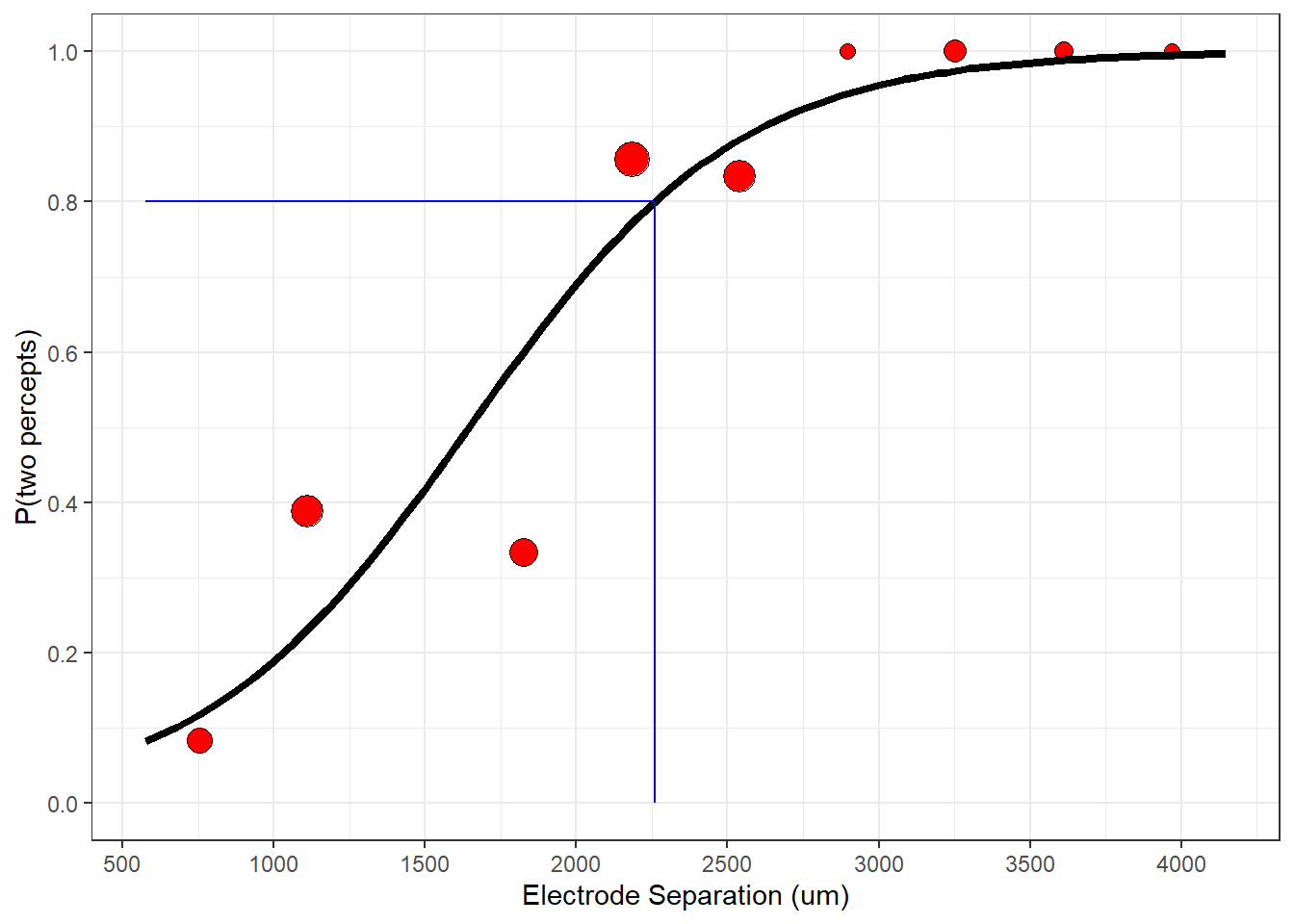
This distance on the retina works out to be about 8 degrees of visual angle, or about the width of about 4 fingers held out at arms-length. That’s pretty big, indicating that this device probably can’t produce high-resolution vision.
Turns out that Second Sight realized this too, and has given up on the Argus II, producing the ethical problem of hundreds of patients with unsupported electronics implanted in their eyes.
24.7 Testing statistical significance: the log-likelihood ratio test
Anyway, let’s discuss statistical significance.
With linear regression we showed that the statistical significance of coefficients can be found using a ‘nested model F test’ which turned out to be numerically identical to the F-statistic from ANOVA. For logistical regression there are a few different methods for getting p-values from our coefficients.
We’ll start with the ‘log-likelihood ratio test’. Like the nested model F test it compares the goodness of fit between ‘complete’ and ‘restricted’ models. For our example, the complete model is the one we just fit with \(\beta_{0}\) and \(\beta{1}\), and the restricted model just has the \(\beta_{0}\) parameter. Sometimes this is called the ‘null’ model:
## [1] 137.4463If the null hypothesis is true, then the difference of the deviances for the two models (or twice the difference between the log-likelihoods) turns out to be distributed as a chi-squared statistic. The degrees of freedom is the difference between the number of parameters.
We can use ‘pchis2’ to get the p-value. There is one degree of freedom because the null model had just the \(\beta_{0}\) parameter, and the full model is the null model plus the \(\beta_{1}\) parameter.
chi_squared <- model_null$deviance - model_dist$deviance
sprintf('chi-squared(%d)= %5.3f',1,chi_squared)
## [1] "chi-squared(1)= 45.051"## [1] "p = 1.91936e-11"There is a very significant effect of distance on the patient’s probability of reporting 2 percepts.
R has it’s own function for the log-likelihood test called ‘lrtest’. If we just send in the complete model it automatically compares it to the null model:
## Likelihood ratio test
##
## Model 1: resp ~ dist
## Model 2: resp ~ 1
##   #Df  LogLik Df  Chisq Pr(>Chisq)
## 1   2 -46.197
## 2   1 -68.723 -1 45.051  1.919e-11 ***
## ---
## Signif. codes:  0 '***' 0.001 '**' 0.01 '*' 0.05 '.' 0.1 ' ' 1
You should recognize these numbers. You’ll see the log-likelihood values (-46.197 and -68.723), the chi-squared value (45.051) which is twice the difference between the log-likelihood values, and the p-value for 1 degree of freedom.
24.8 Adding factors
Just as with linear regression we can fit more complicated models by adding independent variables to the logistic regression model.
A second potentially influential factor is the amplitude of the current used for stimulation, which is the field ‘amp’ in the data frame. Each factor has it’s own coefficient, and each factor adds linearly to the predicted log odd ratio. The model incorporates the next factor \(\beta_{2}\) like this:
\[ y = \beta_{0} + \beta_{1}x_{1} + \beta_{2}x_{2} \]
\(x_{1}\) is distance, as before, and \(x_{2}\) is current amplitude. As before, y is passed through the logistic function to predict the probability of getting ‘1’.
\[ p = \frac{1}{1+e^{-y}} \] R’s glm function incorporates addtional factors just like ‘lm’;
To test the statistical significance of adding this second factor we use the log-likelihood test to compare this fit to the fit using the distance alone. This time we’ll send in the results of both models, since we’re not using the null model.
## Likelihood ratio test
##
## Model 1: resp ~ dist + amp
## Model 2: resp ~ dist
##   #Df  LogLik Df Chisq Pr(>Chisq)
## 1   3 -44.819
## 2   2 -46.197 -1 2.756    0.09689 .
## ---
## Signif. codes:  0 '***' 0.001 '**' 0.01 '*' 0.05 '.' 0.1 ' ' 1
It turns out that current amplitude does not significantly improve the fit (after including distance as a factor).
Do you remember the issue with Type I and Type II ANOVA’s? For unbalanced designs with multiple factors, the order that you add the factors can matter. The same is true for logistic regression. This means that if we want to test the significance of distance while including amplitude, we need to fit the model to amplitude alone first, and then compare that to the complete model:
## Likelihood ratio test
##
## Model 1: resp ~ dist + amp
## Model 2: resp ~ amp
##   #Df  LogLik Df  Chisq Pr(>Chisq)
## 1   3 -44.819
## 2   2 -67.711 -1 45.782  1.322e-11 ***
## ---
## Signif. codes:  0 '***' 0.001 '**' 0.01 '*' 0.05 '.' 0.1 ' ' 1
Distance is still statistically significant - though the p-value is different than before where we simply added distance to the null model. With both amplitude an distance as factors, we should report this last p-value since it’s the result with adding distance last.
You can get R to run a type II log-likelihood ratio test using the Anova function (with the capital A):
## Analysis of Deviance Table (Type II tests)
##
## Response: resp
##      LR Chisq Df Pr(>Chisq)
## dist   45.782  1  1.322e-11 ***
## amp     2.756  1    0.09689 .
## ---
## Signif. codes:  0 '***' 0.001 '**' 0.01 '*' 0.05 '.' 0.1 ' ' 1
Notice the p-values for dist and amp match those from our analyses when the factor is added last.
24.9 Wald test
There are other ways to calculate p-values with logistical regression. A common method is the Wald test. This is the default method in R using the ‘summary’ function:
| Estimate | Std. Error | z value | Pr(>|z|) | |
|---|---|---|---|---|
| (Intercept) | -6.5436795 | 2.0399385 | -3.207783 | 0.0013376 |
| dist | 0.0024604 | 0.0005141 | 4.785509 | 0.0000017 |
| amp | 0.0058554 | 0.0035981 | 1.627361 | 0.1036605 |
Notice that the p-values are similar to those from the log-likelihood ratio test. I’ll confess that don’t know exactly how to go from the raw data to the z-scores for Wald’s test. I do know that Wald’s test is an approximation for the likelihood ratio test. I have no idea why the more complicated Wald test is often the default for logistical regression when it’s an approximation to a simpler likelihood ratio test. From my reading on the topic, we should be using the likelihood ratio test for logistical regression.