Chapter 12 The Binomial Distribution
So far, we have focused on the sampling distribution of means. In this chapter, we consider a different kind of random variable: the number of successes in a fixed number of independent trials. This leads us to the binomial distribution — a discrete probability model that underlies many categorical tests.
When you flip a coin there are only two possible outcomes - heads or tails. This is an example of a dichotomous event. Other examples are getting an answer right vs. wrong on a test, catching vs. missing a bus, or eating vs. not eating your vegetables. A roll of a dice, on other hand, is not a dichotomous event since there are six possible outcomes.
If you flip a coin repeatedly, say 10 times, and count up the number of heads, this number is drawn from what’s called a binomial distribution. Other examples are counting the number of correct answers on an exam, or counting the number of days that your ten year old eats his vegetables at dinner. Importantly, each event has to be independent, so that the outcome of one event does not depend on the outcomes of other events in the sequence.
We can define a binomial distribution with three parameters:
P is the probability of a ‘successful’ event. That is the event type that you’re counting up - like ‘heads’ or ‘correct answers’ or ‘did eat vegetables’. For a coin flip, P = 0.5. For guessing on a 4-option multiple choice test, P = 1/4 = .25. For my twelve year old eating his vegetables, P = 0.05.
N is the number of independent events.
k is the number of ‘successful’ events out of N.
The probability of obtaining k successful events out of N, with probability P is:
\[\frac{N!}{k!(N-k)!} P^{k}(1-P)^{N-k}\]
where N! = \(N(N-1)(N-2)...\), or N ‘factorial’.
12.1 Coin flip example
For example, if you flip a fair coin (P=0.5) 5 times, the probability of getting 2 heads is:
\[Pr(k=2) = \frac{5!}{2!(5-2)!}(0.5)^{2}(1-0.5)^{(5-2)} = (10)(0.5^{2})(0.5)^{3} = 0.3125\]
12.2 R’s dbinom function
R has a function that works like: dbinom(k,N,P). For our example it works like this:
## [1] 0.3125You can send in a list of values into dbinom to get a list of probabilities. Here’s how to get the whole binary frequency distribution:
## [1] 0.03125 0.15625 0.31250 0.31250 0.15625 0.03125We can plot this binomial frequency distribution as a bar graph, highlighting k = 2 in blue:
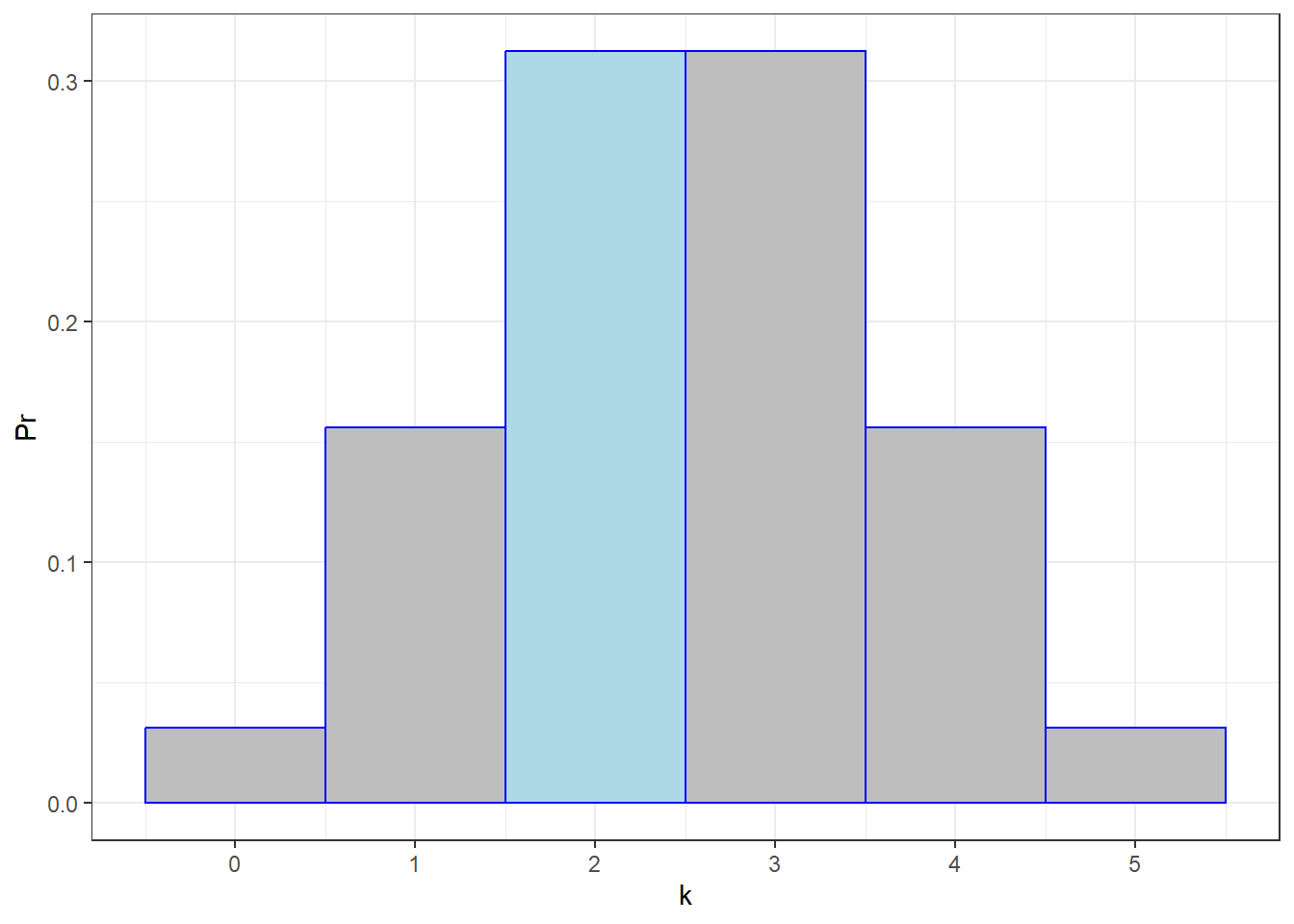
The shape of the probability distribution for N=5 should look familiar. It looks normal! More on this later.
We just calculated the probability of getting exactly 2 heads out of 5 coin flips. What about the probability of calculating 2 or more heads out of 5? It’s not hard to see that:
\[Pr(k \ge 2) = Pr(k=2) + Pr(k=3) + Pr(k=4) + Pr(k=5)\] Which for our example is:
\[0.3125+0.3125+0.15625+0.03125 = 0.8125\]
This is called the ‘cumulative binomial probability’. The easiest way to calculate this with R is to sum up the individual binomial probabilities:
## [1] 0.8125Which can be shown as:
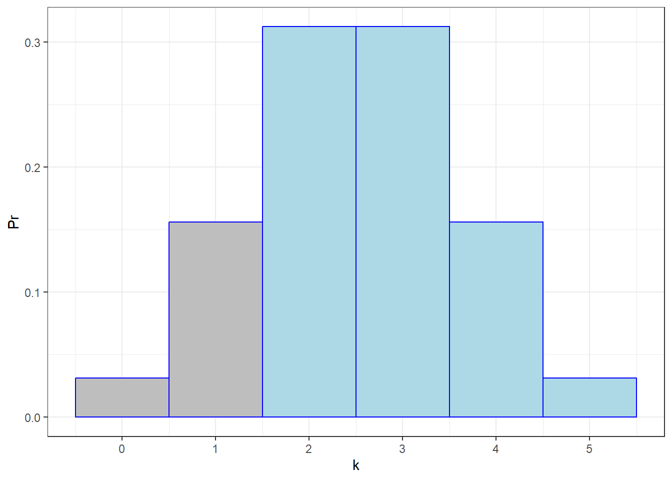 Since each of these bars has a width of 1 unit, the area of each bar represents the probability of each outcome. The total area shaded in blue is therefore \(Pr(k \ge 2)\).
12.3 Exam guessing example
Suppose you’re taking a multiple choice exam in PHYS 422, “Contemporary Nuclear And Particle Physics”. There are 10 questions, each with 4 options. Assume that you have no idea what’s going on and you guess on every question. What is the probability of getting 5 or more answers right?
Since there are 4 options for each multiple choice question, the probability of guessing and getting a single question right is P = \(\frac{1}{4} = 0.25\). The probability of getting 5 or more right is \(Pr(k>=5)\). We can find this answer using dbinom in R with N = 10, k = 5 and P = 0.25:
## [1] 0.07812691What is the probability of getting 6 or fewer wrong? The probability of getting any single problem wrong by chance is 1-0.25 = 1-0.25. We calculate Pr(k \(\le\) 6) with:
## [1] 0.224124912.4 using pbinom to add up probabilities
R’s dbinom gives you the probability of exactly k out of N events. Above we calculated the probability of k or fewer events by summing up probabilities for k, k-1, etc. R has it’s own shortcut for this called pbinom. By default it calculates the probability of k or fewer events, but this default can be reset with the lower.tail input. For our example above, we can calculate the probability of 6 or fewer events out of 10 like this:
## [1] 0.224124912.5 Normal approximation to the binomial
Here’s the probability distribution for P = 0.5 and N = 20:
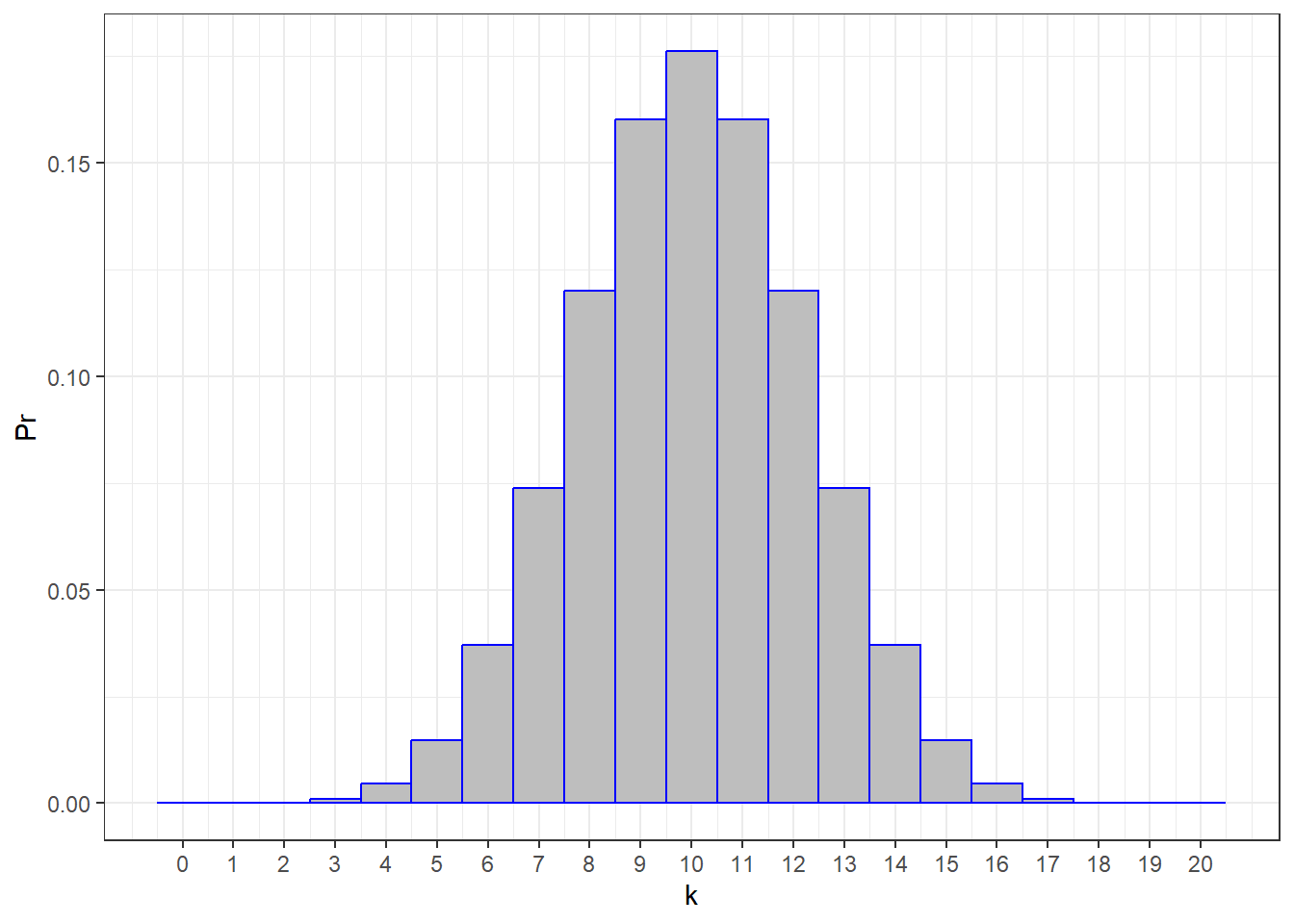
This is a familiar shape! Yes, even though the binomial distribution is ‘discrete’, it’s still shaped like the normal distribution. In fact, we know the mean of the distribution is:
\[ \mu = NP\]
This should make sense. If, for example, you flip a 50/50 coin 100 times, you expect to get (100)(.5) = 50 heads (or tails). For the example above with P = 0.5 and N = 20, \(\mu\) = (20)(0.5) = 10.
Interestingly, the standard deviation is also known:
\[\sigma = \sqrt{NP(1-P)}\] For example, \(\sigma\) = \(\sqrt{(20)(0.5)(0.5)}\) = \(2.2361\)
Here’s that binomial distribution drawn with a smooth normal distribution with \(\mu\) = 10 and \(\sigma\) = 2.2361:
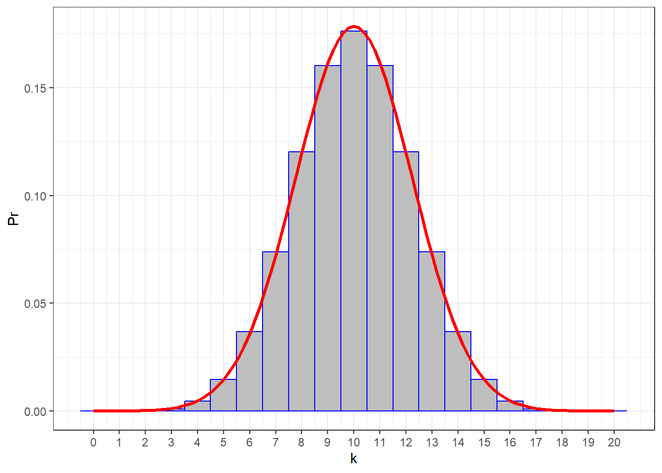 You can see that it’s a nice fit.
If we consider this as the distribution for obtaining k heads out of 20 coin flips, the probability of getting, say 13 or more heads is:
## [1] 0.131588As we mentioned above, you can think of the areas of the gray bars as representing probabilities. So the area under the red normal distribution should be a good approximation to the binomial distribution.
There’s one small adjustment, called the ‘correction for continuity’. Let’s zoom in on the upper tail, shading in the bars for k \(\ge\) 13:
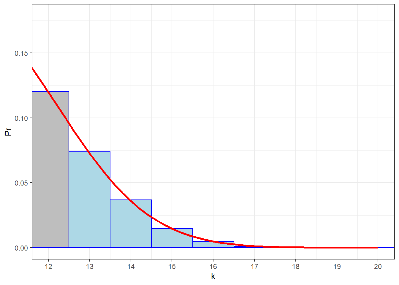 In order to find the area under the (red) normal distribution that approximates the blue area, we need to actually find the area that covers the entire bar for k = 13. That means we need to back up one half of a unit and find the area above k = 12.5. Here’s that area, using
 pnorm:
## [1] 0.1317797This is really close to the result we got from dinom: 0.131588
Using the normal distribution to approximate binomial probabilities used to be really useful when we had to rely on tables for the binomial distribution. Tables typically went up to only N=15 or N=20. But now with computers we can calculate the ‘exact’ probabilities with dinom or its equivalent in other languages.
However, we still rely on this sort of approximation for some statistical tests, like the \(\chi\)-squared test. So it’s good to keep in mind that the \(\chi\)-squared test is actually doing something like the approximation shown above - though often the correction for continuity is left out!
12.6 The binomial hypothesis test: Seattle Mariners season
As of last night as I update this book, the Seattle Mariners have just completed their 2025 season. This record was good enough to give them the lead in their Division and a direct route to the playoff Division Series, bypassing the wildcard series. The Mariners have made the playoffs only one other time since 2001, so local baseball fans are excited. This could be our year!
At the end of the season they won 90 games and lost 72 games. How good is this? Specifically, let’s answer the question: If the Mariners were a truly average team, meaning that there’s a 50% chance of winning any game, what is the probability of having a season this good or better?
This is easy using pbinom. Note that we’re using the default ‘lower.tail’ = TRUE, which finds the probability of wins or less events. So to find the probability of k or more we need to find 1 minus the probability of wins-1 or less events:
wins <- 90 # wins
losses <- 72 # losses
P <- .5  # expected P(win)

N <- wins+losses  # no ties in baseball!

p.value <- 1-pbinom(wins-1,N,P)
p.value
## [1] 0.09074494A totally average team that has a 50/50 chance of winning any game will have a season this good or better 9 percent of the time.
This is a kind of low probability, but above our magic value of 5%. So in terms of hypothesis testing, we cannot conclude that the Mariners’ record is significantly better than chance - despite winning the division. I find this a little depressing. It seems that there is so much randomness in baseball that even the divison winner isn’t significantly better than a series of 162 coin flips.
To get to the magical p<.05, a baseball team needs to win 94 or more games out of 162. (Try it yourself: ``This year, only four teams out of 30 achieved this. If baseball were completely random, we’d expect 5% of the 30 teams, or 1.5 teams to do this by chance. So at least there’s some evidence that the 2430 games played this year pulled some signal out of the noise.
Notice that even there are a large number of games in a season (162), we can still use the binomial distribution. We’re adding up many small numbers, but computers don’t complain about these things.
R has it’s own function for computing a hypothesis test on binomial distributions, called binom.test. It works like this, using the variables from above:
## [1] 0.09074494This is probably a really short function, and we know exactly what it did. In fact, you can use binom.test to get your summed binomial probabilities instead of sum(dbinom(.. like we’ve been doing this chapter.
You can set alternative = 'two.sided, which is the default, which effectively doubles the p-value. It tests the hypothesis of obtaining a value of k that is far away from nP in either direction. If we want to see if the Mariner’s season is truly exceptional, we really should have run a two-tailed test. In this case, the p-value is p = 0.1815. With a p-value around 0.5, this means that the 2024 Mariners aren’t even unusually average, if that makes any sense.
12.7 The margin of error in polling
You’ve all seen the results of a poll where an article will state that the ‘results are within the margin of error’. What does this mean? Consider a poll where there are two choices, candidate D and candidate R. Suppose that in the population, 50 percent of voters are planning on voting for candidate D and 50 percent of voters are planning on voting for candidate R.
If we sample 1000 voters from the population, then using the normal approximation to the binomial, we know that the the number of voters for candidate D will be distributed normally with a mean of
\[ \mu = NP = (1000)(0.5)=500\] and a standard deviation of
\[ \sigma = \sqrt{NP(1-P)} = \sqrt{(1000)(0.5)(0.5)} = 15.811\]
Polls, however, are reported in terms of the proportions or percentages, not in terms of the number of voters preferring a candidate. We can convert the counts of voters to percentage of voters by dividing the equations above by total sample size and multiplying by 100. Remember, when we multiply (or divide) the scores in a normal distribution by a constant, both the mean and standard deviation are multiplied (or divided) by that same constant. So (not surprisingly) the percent of voters in the poll will be drawn from a normal distribution with mean:
\[ \mu_{percent} = 100\frac{NP}{N} = (100)(0.5)= 50\]
and a standard deviation of:
\[ \sigma_{percent} = 100\frac{\sqrt{NP(1-P)}}{N} = 100\sqrt{\frac{P(1-P)}{N}} = 100\sqrt{\frac{(0.5)(1-0.5)}{1000}} = 0.0158\]
When pollsters talk about the “margin of error,” they are referring to a confidence interval. By default—unless otherwise specified—a confidence interval covers 95% of the sampling distribution. Since
this is a normal distribution, we can use qnorm to calculate the 95% confidence interval for our poll:
N <- 1000
P <- .5
alpha <- .05
sigma_percent <- 100*sqrt((P*(1-P))/N)
CI = qnorm(1-alpha/2,0,sigma_percent)
sprintf('Our margin of error is plus or minus %0.2f percentage points',CI)
## [1] "Our margin of error is plus or minus 3.10 percentage points"The margin of error depends both on P and on the sample size, N. For close races, we can assume that P = 0.5. Here’s a graph of how the margin of error depends on the sample size:
From this graph you can estimate the sample size of a poll from the reported margin of error. You’ve probably noticed that typical polls have a margin of error of around 2-3 percentage points. You can tell from the graph that this is because typical polls have around 1000-2000 voters.
You can also appreciate the diminishing returns with increasing poll size. A poll of N = 100 has nearly a 10% confidence interval, but once you get to 1000 you’re down to 3%, and it decreases slowly from there.