Chapter 7 One Sample T-Test
The one sample t-test is used to compare a single mean to an expected mean under the null hypothesis when you don’t know the standard deviation of the population.
You can find this test in the flow chart here:

7.2 Simulating z-scores: replacing the population s.d. with the sample s.d.
See if you can follow what’s going on in this R-code:
nSamples <- 30000
mu <- 100
sigma <- 15
n <- 5  # sample size
t = numeric(nSamples)
z = numeric(nSamples)
for (i in 1:nSamples) {
  # draw a sample of size n from a normal distribution
  samp <- rnorm(n,mu,sigma)
  # calculate the z-statistic for this sample using the the population s.d.
  z[i] <- (mean(samp)-mu)/(sigma/sqrt(n))
  # calculate the t-statistic for this sample using the sample s.d.
  t[i] <- (mean(samp)-mu)/(sd(samp)/sqrt(n))
}
The code uses a for loop to generate 30000 samples of of size 5 drawn from a normal distribution using R’s dnorm function. For each sample, a z-score is calculated by subtracting the population mean and dividing by the standard error of the mean using the known population standard deviation:
\[ z = \frac{(\bar{x}-\mu_{hyp})}{\sigma_{\bar{x}}} \]
where:
\[ \sigma_{\bar{x}} = \frac{\sigma}{\sqrt{n}} \] But what if we don’t know the population standard deviation? This is really the more common situation. After all, we’re trying to make an inference about the population so it’s unlikely that we know that much about it.
If we don’t know the population standard deviation it might make sense to use the standard deviation of our sample instead. After all, the sample standard deviation \(s_{x}\) is an unbiased estimate of the population standard deviation \(\sigma_{x}\).
In the code, a score like the z-score is also calculated, but instead dividing by the standard error of the mean using the sample standard deviation. We call this score ‘t’ instead of ‘z’ because you’ll see in a second that it’s not the same thing. Formally, ‘t’ is calculated as:
\[ t = \frac{(\bar{x} - \mu_{hyp})}{s_{\bar{x}}} \] Where, just like for \(\sigma_{x}\) but using the sample standard deviation:
\[ s_{\bar{x}} = \frac{s}{\sqrt{n}} \]
If all goes well, a histogram of the z-scores should match well with the standard normal distribution. Here’s a histogram of the 30000 z-scores along with the smooth standard normal distribution:
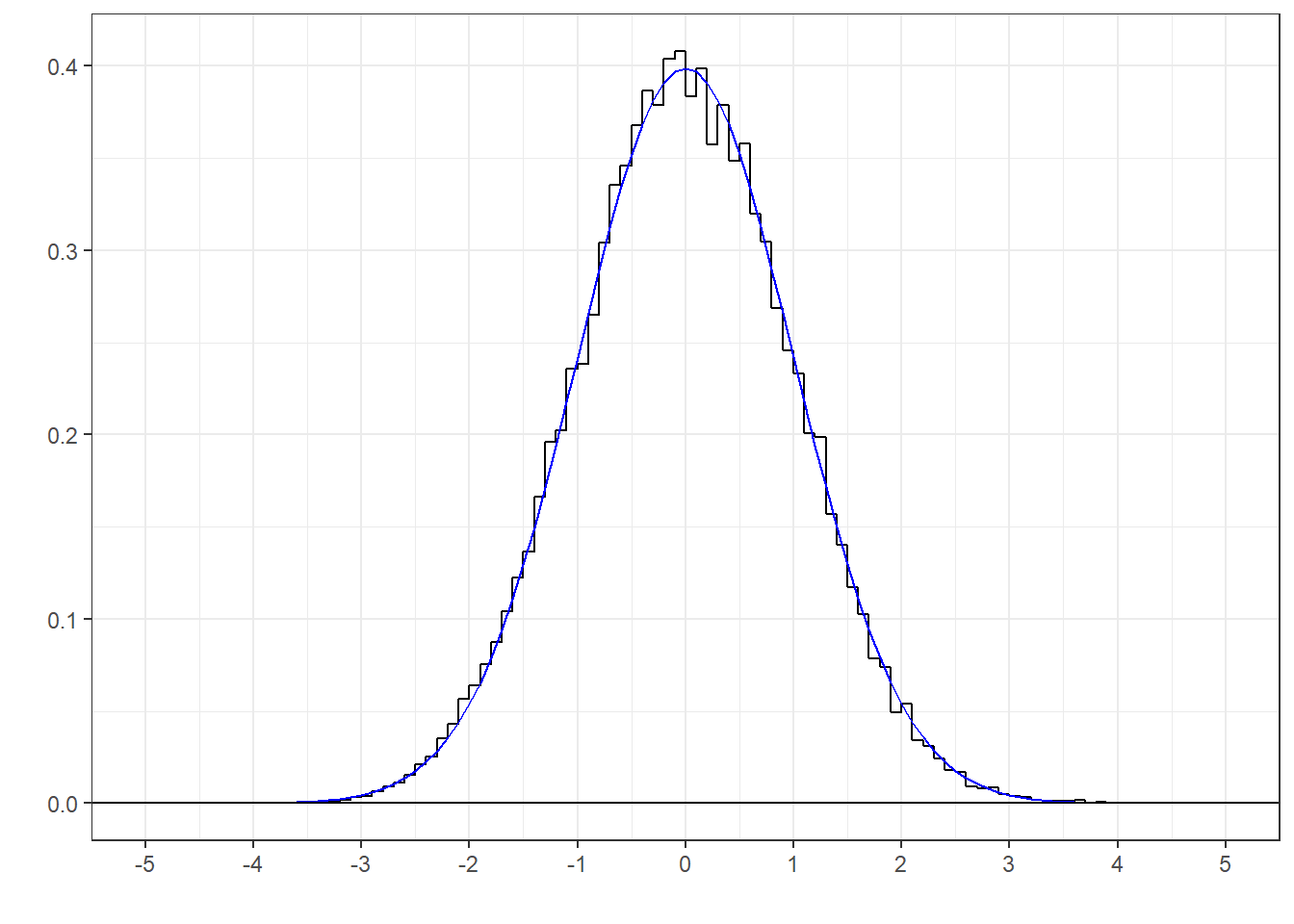
It looks like a good fit. This means that if we use a known population standard deviation, and the null hypothesis is true, then when we convert our observed mean to a z-score we can use the standard normal distribution (pnorm in R) to calculate our p-values.
But here’s a histogram of the ‘t’ scores along with the standard normal distribution:
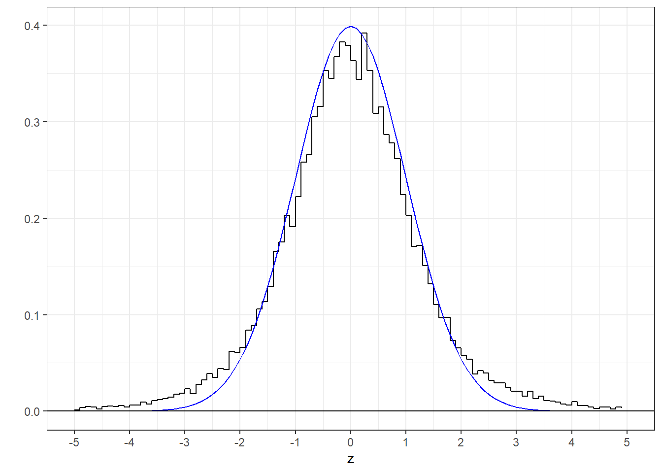
This is not a good fit. Notice the fat tails in the t-distribution compared to the standard normal, or z-distribution. This is because while the standard deviation of each sample may be an unbiased estimate of the population standard deviation, it is still a ‘random variable’, meaning that it varies from sample to sample. Sometimes, by chance, \(s_{x}\) will be small compared to \(\sigma_{x}\) so the t-statistic will end up large. If we were to use the standard normal distribution to calculate our p-values, we’d end up landing in the rejection zone way too often by accident.
7.3 The t-distribution
This distribution of ‘t’ scores has a known shape. It’s much like a normal distribution but it has longer tails. It also varies with sample size. As the sample size increases, the estimate of the population standard deviation gets more accurate (like a Central Limit Theorem for standard deviations). This makes the t-distribution look more like the z-distribution with larger sample sizes.
R’s function for calculating areas or probabilities for the t-distribution is called ‘pt’ and it’s inverse, ‘qt’, and have the same functionality as ‘pnorm’ and ‘qnorm’ for the normal distribution. The main difference is that ‘pt’ and ‘qt’ needs to know something about the sample size, or more specifically the ‘degrees of freedom’ which is the sample size minus one when we’re dealing with one mean. Here’s a histogram of our sampled t-scores and the known t-distribution for 5-1 = 4 degrees of freedom:
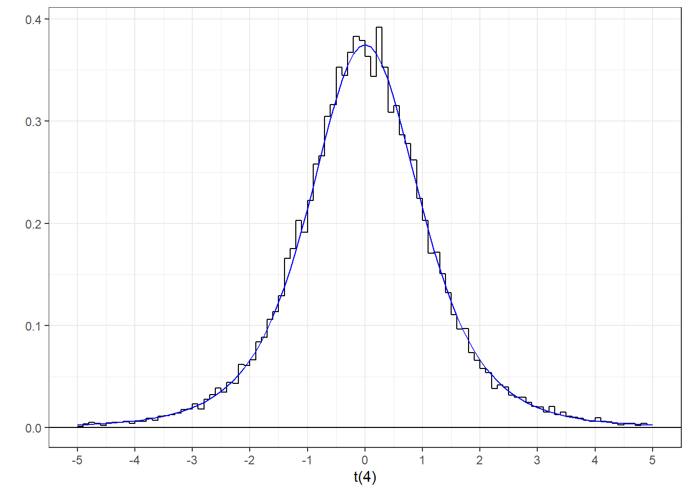 That’s more like it. The ‘t(4)’ x-axis label indicates that this is a t-distribution with 4 degrees of freedom.
Since the t-distribution depends on the sample size, the t-distribution is actually a ‘family’ of distributions, one for each sample size. Specifically, we define each separate t-distribution by its ‘degrees of freedom’, df, which for a single mean is df = n-1. Here are some example t-distributions:
 You can see how the t-distribution starts out with fat tails for 4 degrees of freedom (df=4) and tightens up with increasing df. By df = 32 the t-distribution is nearly identical to the z-distribution.
You can also see this by comparing the area above, say 2, for z and various t-distributions using R:
## [1] 0.02275013## [1] 0.05805826 0.04025812 0.03138598 0.02702409About 2.3% of the area under the z-distribution lies above z=2, but 5.8% lies above the t-distribution for t=2 for df=4. But with df = 32, the area drops down to 2.7% which is getting close to the area for the z-distribution.
7.4 Example: Blood pressure and PTSD
Suppose you want to see if patients with PTSD have higher than normal systolic blood pressure. You sample 25 patients and obtain a sample mean Systolic BP of 124.22 and a sample standard deviation of 23.7527 mm Hg. Using an alpha value of 0.05 is this observed mean greater than a ‘normal’ Systolic BP of 120 mm Hg?
Like the z-test, we first compute the standard error of the mean, but using the sample standard deviation:
\(s_{\bar{x}} = \frac{s_{x}}{\sqrt{n}} = \frac{23.7527}{\sqrt{25}} = 4.7505\)
We then calculate our t-statistic by subtracting the mean for the null hypothesis and divide by the estimated standard error of the mean:
\(t = \frac{(\bar{x} - \mu_{H0})}{s_{\bar{x}}} = \frac{124.22-120}{4.7505} = 0.8876\)
Since we’re only rejecting \(H_{0}\) for high values, this is a one-tailed test. We need to find the p-value, which is the probability of obtaining a score of 0.8876 or higher from the standard t-distribution. Since the sample size is 25, there are \(df = 24\) degrees of freedom. Here’s how to get this p-value:
## [1] 0.1917825Our p-value of 0.1918 is greater than \(\alpha\) = 0.05, so we fail to reject \(H_{0}\) and conclude that our patients with PTSD do not have significantly higher than normal systolic blood pressure.
7.5 Example from the survey: Men’s heights compared to 5’10”
Let’s test the hypothesis that the average height of men in Psych 315 is different from an expected height of 70 inches (5’10”) using a \(\alpha\) = 0.05. We’ll do this with R in two ways.
7.5.1 By hand
First we’ll conduct the test ‘by hand’ by calculating the t-statistic using the sample mean and standard deviation:
x <- na.omit(survey$height[survey$gender == "Man"])
n <- length(x)
df <- n-1
m <- mean(x)
sprintf('mean = %5.4f',m )
## [1] "mean = 70.3103"## [1] "standard devation = 3.1521"## [1] "standard error of the mean = 0.5853"## [1] "t(28)=0.5302"The code above calculates that \(n = 29\), \(\bar{x} = 70.3103\), \(s = 3.1521\) and \(s_{\bar{x}} = 0.5853\).
From these values, the t-statistic was found to be:
\(t = \frac{(\bar{x} - \mu_{H0})}{s_{\bar{x}}} = \frac{70.31-70}{0.5853} = 0.5302\)
From t=0.5302 and df = 28 we can use R’s ‘tp’ function to find our p-value. Note that we’ll be rejecting \(H_{0}\) if there is a significant difference between our mean and 70 inches, so this is a two-tailed test. That means we will be doubling the area under t-distribution beyond our observed value of t. Here’s one way of doing it in R:
## [1] "p = 0.6002"Let’s unpack this working from the inside out. First we take the absolute value of t since with a two-tailed test we really only care about how far t is away from zero. This way, ‘1-(abs(t),df)’ finds the area above the absolute value of t. We then double this area to find the p-value for a two-tailed test.
Our p-value of 0.6002 is greater than \(\alpha\) = 0.05, so we fail to reject \(H_{0}\) and conclude that the average height of men is not significantly different from 70 inches.
7.5.2 Using t.test
Now we introduce our first function in R for conducting a hypothesis test using actual data (and not just summary statistics). R’s ‘t.test’ function goes through the same steps that we just did by hand. ‘t.test’ is also used to compare two means, which we’ll cover in the next chapter.
If you use R’s help function (using, at the Console, ‘?’followed by ’t.test’) to investigate how to use t.test you’ll see:
t.test(x, y = NULL, alternative = c(“two.sided”, “less”, “greater”), mu = 0, paired = FALSE, var.equal = FALSE, conf.level = 0.95, …)
The first argument sent into t.test,‘x’, is a vector containing the data, which is the minimum amount of information needed. The rest are set to defaults which you can set. The second argument ‘y’ is a second vector for a ‘two-sample’ t.test. When used, t.test will run a hypothesis test comparing the means of x and y. ‘alternative’ is used to run either a one or a two-tailed test (the default), and “less” vs. “greater” tells the function which direction to reject \(H_{0}\). ‘mu’ is the mean for the null hypothesis - the value that will be compared to our sample mean. ‘paired’ and ‘var.equal’ are for two-sample t.tests which we’ll cover in the next chapter.
Here’s how to run the test on Man heights using t.test:
##
##  One Sample t-test
##
## data:  x
## t = 0.5302, df = 28, p-value = 0.6002
## alternative hypothesis: true mean is not equal to 70
## 95 percent confidence interval:
##  69.11134 71.50935
## sample estimates:
## mean of x
##  70.31034
You should see some familiar numbers here that match the values we calculated by hand including the p-value. Hopefully you’ll appreciate that the ‘t.test’ function isn’t doing something too mysterious and is instead doing something we’ve done by hand.
Running ‘t.test’ spits out the results into your console. It’s sometimes useful to have access to these values as variables so you don’t have to copy them from the console. This can be done by sending the output of t.test into an ‘object’ like this:
I’ve used the variable name ‘out’ but you can call it anything you’d like. When you run this the results are stored into ‘out’ and nothing is dumped into the console. To investigate what’s in there, you can type ‘out$’ at the console and you’ll see a list of fields that have been filled in. For example, the p-value is found in:
## [1] 0.60015417.6 APA style
APA has a specific style for reporting the results of a t.test. The style includes the mean, standard deviation, degrees of freedom and p.value:
t(degrees of freedom) = the t statistic, p = p value
We can use ‘sprintf’ to convert the output of the t.test in ‘out’ into a string containing the results in APA style:
## [1] "t(28)=0.5302, p = 0.6002"To report the results in the context of the experiment, including the mean and standard deviation. To start, let’s pull out the important numbers that can be found in ‘out’:
m <- out$estimate     # mean
t <- out$statistic    # t-value
p <- out$p.value      # p-value
df <- out$parameter   # degrees of freedom
sem <- out$stderr     # standard error of the mean
H0 <- out$null.value  # null hypothesis mean
For some reason, t.test doesn’t give you the standard deviation of the sample (\(s_{x}\)), but it does give you the standard error of the mean (\(s_{\bar{x}}\)). It also doesn’t give you the sample size, but it does give you the degrees of freedom. The sample size is just \(n= df+1\), and since \(s_{\bar{x}} = \frac{s_{x}}{\sqrt{n}}\), \(s_{x} = s_{\bar{x}}\sqrt{n}\)
From all this, we can generate a string containing our results:
str <- sprintf('The height of the men in Psych 315 (M = %5.4f, S = %5.4f) is not significantly different from %g inches, t(%d)=%5.4f, p = %5.4f',m,s,H0,df,t,p)## [1] "The height of the men in Psych 315 (M = 70.3103, S = 3.1521) is not significantly different from 70 inches, t(28)=0.5302, p = 0.6002"