Chapter 9 Power
9.1 Definition of power
If you retain anything from this class, it should be the following definition of power:
Power is the probability of correctly rejecting the null hypothesis.
I suggest you repeat this to yourself so this definition reflexively pops into your head whenever you read or hear about statistical power.
The word ‘correctly’ is doing the heavy lifting here. If you correctly reject the null hypothesis, the null hypothesis must be false. So power is the probability of detecting an effect only if there truly is one.
In this chapter we’ll define what this means in the context of a specific example: a z-test on the mean of a sample of IQ scores. This first part should be a review for you.
9.2 Z-test example
Suppose you want to test the hypothesis that the mean IQ of students at UW have a higher IQ than the population that has a mean IQ of 100 points. We also know that the standard deviation of the IQ’s in the population is 15.
You measure the IQ in 9 UW students and obtain a mean IQ of 106. First we’ll determine if this mean is significantly greater than 100 using \(\alpha\) = 0.05.
To conduct this test we need to calculate the standard error of the mean and then convert our observed mean into a z-score:
\[ \sigma_{\bar{x}} = \frac{\sigma_{x}}{\sqrt{n}} = \frac{15}{\sqrt{9}} = 5 \]
and
\[ z=\frac{(\bar{x}-\mu_{H_0})}{\sigma_{\bar{x}}} = \frac{(106-100)}{5} = 1.2\]
With a one-tailed test and \(\alpha\) = 0.05, the critical value of z is \(z_{crit}\) = 1.64. Since our observed value of z=1.2 is less than the critical value of 1.64 we fail to reject \(H_{0}\) and conclude that the mean IQ of UW students is not significantly greater than 100.
9.2.1 When the \(H_{0}\) is false
Remember, if \(H_{0}\) is false then the probability of rejecting \(H_{0}\) is the power of our test. How do we find power?
To calculate power we need to know the true mean of the population, which is different than the mean for \(H_{0}\). This probably seems weird to you. If we knew the true mean then we wouldn’t have to run an experiment in the first place.
Since we don’t know the true mean of the distribution we play a ‘what if’ game and calculate power for some hypothetical value for the true mean. For our example, let’s suppose that the true mean is equal to the observed mean of \(\bar{x}\) = 106.
We just calculated that our observed mean of \(\bar{x}\) = 106 converts to a z-score of z = 1.2. So if we assume that the true mean IQ score is \(\mu_{true}\) = 106, then our z-scores will be drawn from a ‘true’ population with mean that I’ll call \(z_{true}\). We’ll assume that the standard deviation \(\sigma_{x}\) is still 15:
\[ z_{true} = \frac{(\mu_{true}-\mu_{H_0})}{\sigma_{\bar{x}}} = \frac{(\mu_{true}-\mu_{H_0})}{\frac{\sigma_{x}}{\sqrt{n}}} =\frac{(106-100)}{\frac{15}{\sqrt{9}}} = \frac{(106-100)}{5} = 1.2 \]
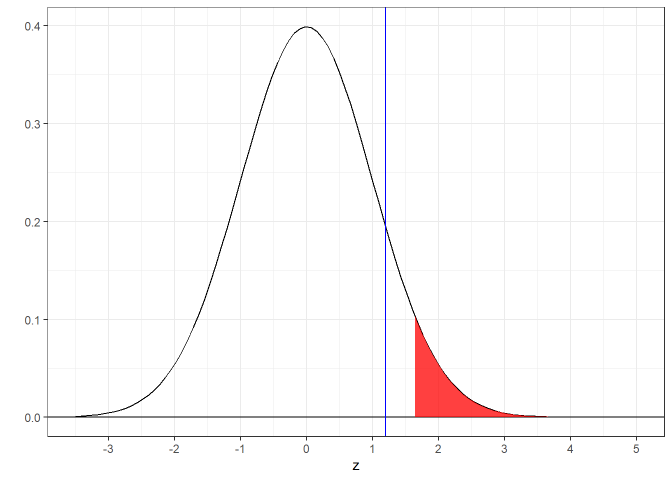
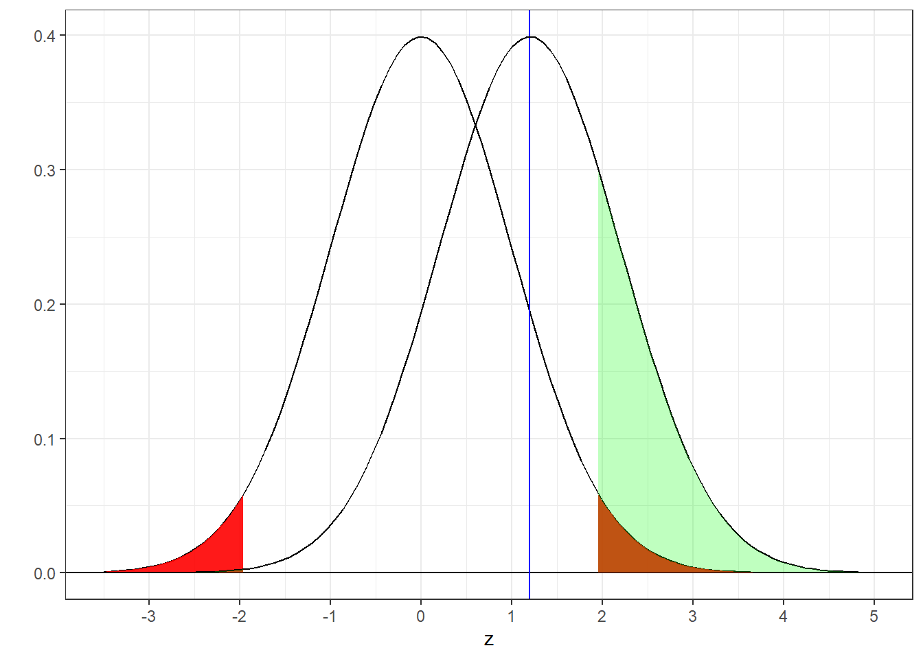
Here’s the true distribution drawn on top of the null hypothesis distribution:
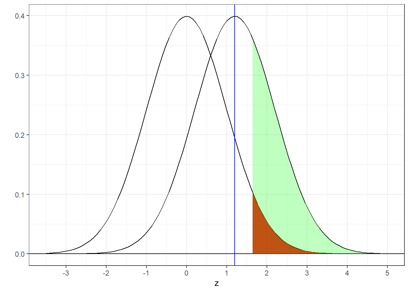
Importantly, even though we`re now drawing z-scores from the ‘true’ distribution, our decision rule remains the same: if our observed value of z is greater than the critical value (z = 1.64 in this example), then we reject \(H_{0}\). I’ve colored this region above z = 1.64 under the ‘true’ distribution in green. Note, the area above 1.64 also includes the red area.
It should be clear that this green area (including the red area) is the power of our hypothesis test. It’s the probability of rejecting \(H_{0}\) when \(H_{0}\) is false. You can see that the green area (power) is greater than the red area (\(\alpha\)). R’s pnorm function will give you this area. It’s the area above 1.64 for a normal distribution centered at 1.2 with a standard deviation of 1:
## [1] 0.3299686So what does a power of 0.33 mean? It means that if the true mean of the population had an IQ of 106, then with our sample size of 9 and \(\alpha\)=0.05, the probability that we’d draw a mean is significantly greater than 100, and therefore correctly reject \(H_{0}\), is 0.33.
9.3 The 2x2 matrix of All Things That Can Happen
Out there in the world, the null hypothesis is either true or it is not true. To make a decision about the state of the world we run an experiment and a following hypothesis test and decide either to reject or to fail to reject the null hypothesis. Therefore, when we run a hypothesis test, there are four possible things that can happen. This can be described as a 2x2 matrix:
| \(H_0\) True | \(H_0\) False | |
|---|---|---|
| Reject \(H_0\) | Error | Correct |
| Fail to Reject \(H_0\) | Correct | Error |
Of the four things, two are correct outcomes (green) and two are errors (red). Consider the case where the null hypothesis is \(H_{0}\) is true. We’ve made an error if we reject \(H_{0}\). Rejecting \(H_{0}\) when it’s actually true is called a Type I error.
9.3.1 Pr(Type I error) = \(\alpha\)
Type I errors happen when we accidentally reject \(H_{0}\). This happens when we draw from the null hypothesis distribution, but happen to grab a mean that falls in the rejection region of the null hypothesis distribution. We know the probability of this happening because we’ve deliberately chosen it - it’s \(\alpha\).
It follows that the probability of correctly rejecting \(H_{0}\) is \(1-\alpha\).
9.3.2 Pr(Type II error) = \(\beta\)
Type II errors happen when we accidentally fail to reject \(H_{0}\). This happens when we grab a mean from the ‘true’ distribution that happens to fall outside the rejection region of the null hypothesis distribution. We have a special greek letter for this probability, \(\beta\) (‘beta’).
9.3.3 power = 1-\(\beta\)
Remember, power is the probability of correctly rejecting \(H_{0}\). This is the opposite of a Type II error, which is when we accidentally fail to reject \(H_{0}\). Therefore, power = 1-Pr(Type II error) which is the same as power = \(1-\beta\).
We can summarize all of these probabilities in our 2x2 table of All Things that Can Happen:
| \(H_0\) True | \(H_0\) False | |
|---|---|---|
| Reject \(H_0\) | Type I Error (\(\alpha\)) | Power (1-\(\beta\)) |
| Fail to Reject \(H_0\) | 1-\(\alpha\) | Type II Error (\(\beta\)) |
For our example, we can fill in the probabilities for all four types of events:
| \(H_0\) True | \(H_0\) False | |
|---|---|---|
| Reject \(H_0\) | 0.05 | 0.33 |
| Fail to Reject \(H_0\) | 0.95 | 0.67 |
9.4 Things that affect power
Figures like the one above with overlapping null and true distributions show up in all textbook discussion of power. Google ‘statistical power’ and check out the associated images. It’s an ubiquitous image because it’s very useful for visualizing how power is affected by various factors in your experimental design and your data.
Looking at the figure, you should see that power will increase if we separate the two normal distributions. There are a variety of ways this can happen.
9.4.1 Increasing effect size increases power
The most obvious way is for us to choose a larger difference between the true mean and the null hypothesis mean. The numerator of Cohen’s d is this this difference between means, so if we have a larger effect size, we’ll have more power.
The effect size in our current example on IQ’s is
\[ \frac{|\mu_{true}-\mu_{H_0}|}{\sigma} = \frac{|106-100|}{15} = 0.4\]
This is a medium effect size.
What if we think that the true distribution has a mean of \(\mu_{true}\) = 112 IQ points? This will increase the effect size to:
\[ \frac{|\mu_{true}-\mu_{H_0}|}{\sigma} = \frac{|112-100|}{15} = 0.8 \]
which is a large effect size.
Means drawn from this new true distribution will have z-scores that are normally distributed with a mean of
\[ z_{true} = \frac{(\mu_{true}-\mu_{H_0})}{\sigma_{\bar{x}}} = \frac{(112-100)}{5} = 2.4\]
Here’s that standard diagram for this new true distribution:
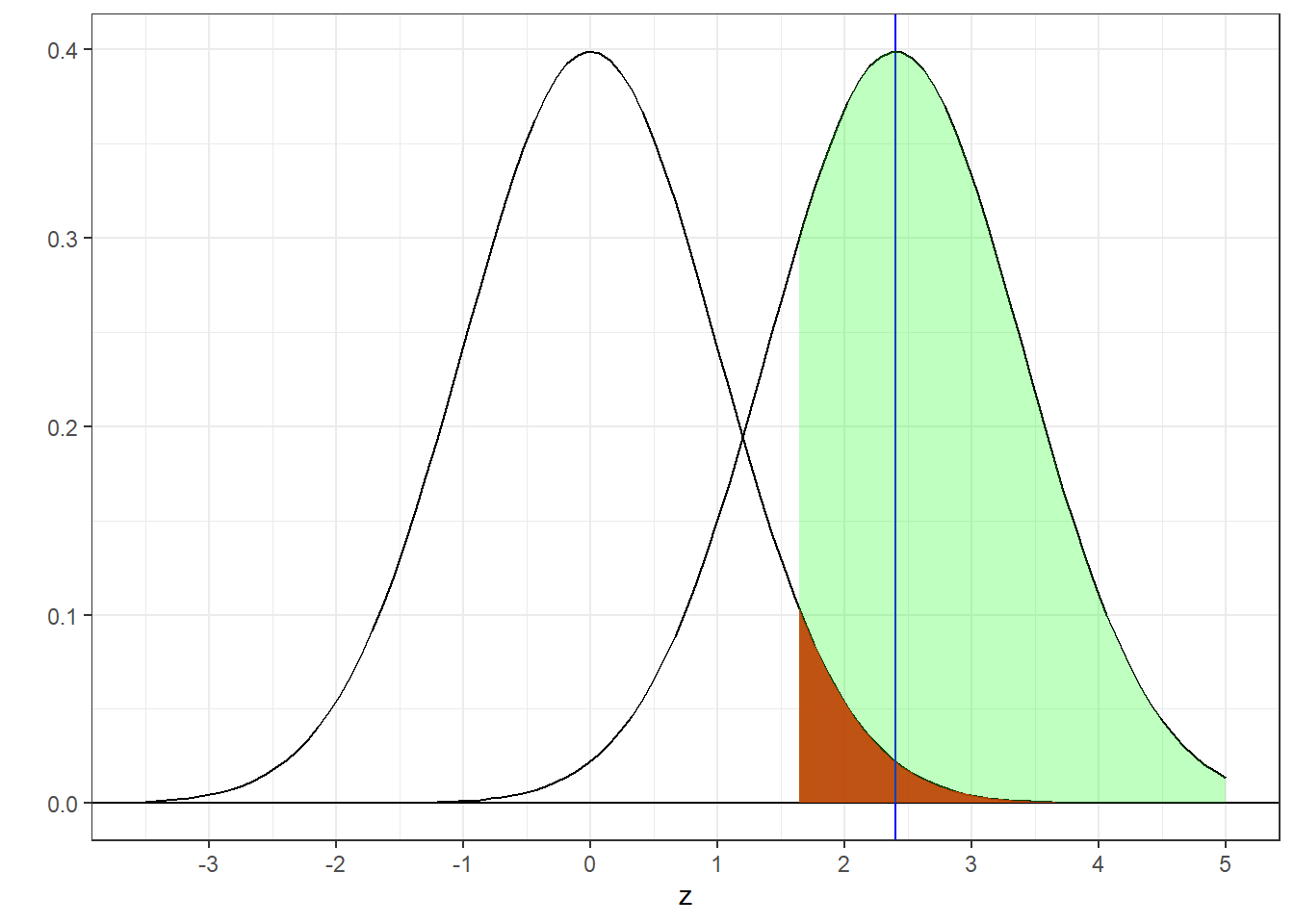
Notice what has changed and what has not changed. The true distribution is now shifted rightward to have a mean of \(z_{true}\) = 2.4. However, the critical region is unchanged - we still reject \(H_{0}\) if our observed value of z is greater than 1.64.
Remember, power is the green area - the area under the true distribution above the critical value of z. You can now see how shifting the true distribution rightward increases power. The power of this hypothesis test is now:
## [1] 0.7763727Increasing the effect size from 0.4 to 0.8 increased the power from 0.33 to 0.7764.
9.4.2 Increasing sample size increases power
Another way to shift the true distribution away from the null hypothesis distribution is to increase the sample size. For example, let’s go back and assume that our true mean IQ is 106 points, but new let’s increase our sample size from 9 to 36. The z-score for the mean of the true distribution is now:
\[ z_{true} = \frac{(\mu_{true}-\mu_{H_0})}{\sigma_{\bar{x}}} = \frac{(\mu_{true}-\mu_{H_0})}{\frac{\sigma_{x}}{\sqrt{n}}} =\frac{(106-100)}{\frac{15}{\sqrt{36}}} = \frac{(106-100)}{2.5} = 2.4\]
This shift in \(z_{true}\) from 1.2 to 2.4 is the same as for the last example where \(\mu_{true}\) was 112 IQ points and a sample size of 9. Thus, the power will also be 0.7749.
Note that increasing sample size increased the power without affecting the effect size (which doesn’t depend on sample size).
effect size: \(\frac{|\mu_{true}-\mu_{H_0}|}{\sigma} = \frac{|106-100|}{15} = 0.4\).
9.4.3 Decreasing \(\alpha\) decreases power
A third thing that affects power is your choice of \(\alpha\). Recall that back in our original example with a mean of 9 IQ scores with \(\mu_{true}\) = 106 points, the power for \(\alpha\) = 0.05 was 0.33.
What if we keep the sample size at 9 so that effect size the same, but decrease our value of \(\alpha\) to our second-favorite value, 0.01?
Decreasing \(\alpha\) from 0.05 to 0.01 increases the critical value of z from 1.64 to 2.33.
Here’s the new picture:
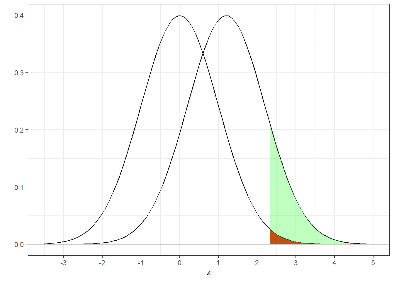
Notice that the true distribution still has a mean of \(z_{true}\) = 1.2. But shifting the critical value of z cuts into the green area. Power is now calculated as:
## [1] 0.1292381The power decreased from 0.33 to 0.1292.
This illustrates a classic trade-off of Type I and Type II errors in decision making. Decreasing \(\alpha\) by definition decreases the probability of making a Type I error. That is, decreasing \(\alpha\) makes it harder to accidentally reject \(H_{0}\). But that comes with the cost decreasing \(\alpha\) also makes it harder to correctly reject \(H_{0}\) if it was true. That’s the same as a decrease in power. and a corresponding increase the probability of a Type II error (\(\beta\)), since power = \(1-\beta\).
Get it? If you`re still following things, when \(\alpha\) goes down, \(z_{crit}\) goes up, power goes down and Pr(Type II error) goes up. whew
9.4.4 Power goes down with two-tailed tests
Let’s look at our power calculation as we shift our original example from a one-tailed to a two-tailed test. Power calculations with two-tailed tests are a little more complicated because we have two rejection regions, but the concept is the same. We’ll keep the true mean at 106 IQ points, the sample size n = 9 and \(\alpha\) = 0.05.
Recall that the critical value of z for a two-tailed test increases because we need to split the area in rejection region in half. You can therefore think of shifting to a two-tailed test as sort of like decreasing \(\alpha\), which as we know decreases power.
Here’s the new picture:
Power is, as always, the area under the true distribution that falls in the rejection region. Now we have two rejection regions, one for z <1.96 and one for z > 1.96. For a two-tailed test we need to add up two areas. For this example, the area in the negative region is so far below the true distribution that the area below z = -1.96 is very close to zero. This leaves the green area above z = 1.96.
The power of a two-tailed test is the sum of two areas:
## [1] 0.2244161Our power is therefore 0.2244. This is lower than the power for the one-tailed test calculated above (0.33).
Here’s a summary of how things affect power:
| Thing | Pr(Type I error) | effect size | power |
|---|---|---|---|
| increasing effect size | same | increases | increases |
| increasing sample size | same | same | increases |
| decreasing alpha | decreases | same | decreases |
| two-tailed test | same | same | decreases |
Go through the table and be sure to understand not only what happens with each thing, but also why.
9.5 Power Widget
Now it’s your turn. You can see for yourself how changing these things affect power with the widget below. You can either slide the bars, type values in or grab objects in the graph. Starting with the original values of \(\sigma = 15\), \(n = 9\), \(\mu_{true} = 106\), \(\mu_{H0} = 100\) and \(\alpha = 0.05\).
If you’re looking at a printout or pdf, you can open the widget here: https://gboynton.github.io/power_z/power_z.html.
See if you can replicate the power values that we calculated above as we adjusted the effect size, sample, size, \(\alpha\) and a one vs. two-tailed tests.
For another exercise, find the difference between the true and null hypothesis means that leads to a power of 0.5. Where is the true mean with respect to the critical value?
9.6 Power for t-tests
This last example used IQ’s and therefore the z-distribution since we know the population standard deviation. Calculating power for t-tests is done conceptually the same way as described above, but with t-distributions instead of z-distributions. Since z’s and t’s look much the same, the pictures with the bell curves look almost identical and all the discussion about things that affect power are still true.
Fortunately, R has a function that does all of this calculation for you. It’s called ‘power.t.test’. Let’s go back to PTSD and blood pressure example from the chapter on t-tests for one mean and discuss the power of that t-test.
9.6.1 PTSD and Blood Pressure Example
Recall that the test was to see if patients with PTSD have higher than normal systolic blood pressure. The sample size was 25 patients, the sample mean Systolic BP was 124.22 and the sample standard deviation was 23.7527 mm Hg. We used an alpha value of 0.05 to test if this observed mean was greater than a ‘normal’ Systolic BP of 120 mm Hg. We ended up failing to reject \(H_{0}\) with a p-value of 0.1918. Using APA format we write:
(M = 124.22, S = 23.7527), t(24) = 0.89, p = 0.1918
To calculate power we need to know the 4 things that affect power: (1) the sample size, (2) \(\alpha\), (3) the effect size, and (4) whether it’s a one or two tailed test.
This where we make something up. How do we know the effect size if we don’t know the true mean of the population? After all, if we knew the true mean, we wouldn’t have to run the experiment in the first place. One guess for the effect size is to use the effect size of our result. This is asking the question: ‘What is the power of our test if the true mean is actually equal to the mean of our sample?’. When we use the effect size from our data we’re calculating what’s called ‘observed power’. Let’s calculate the observed power from our example. We first have to calculate the effect size from our results by hand:
\[d = \frac{|\overline{x} - \mu_{H0}|}{s_{x}} = \frac{124.22-120}{23.7527} = 0.1775\]
This is a small effect size.
Here’s how to use power.t.test find the observed power for this last example.
power.out <- power.t.test(n=25,delta=0.1775,sig.level=0.05,type ='one.sample',alternative = 'one.sided')Most of the inputs are self explanatory. For some reason, ppwer.t.test uses the name ‘delta’ for effect size. ‘sig.level’ is where we put in our value of \(\alpha\). The only new thing here is ‘type’ which is ‘one.sample’ for this example because this is a t-test for one mean. In the next chapter we’ll comparing two means, so we’ll use ‘two.sample’ for ‘type’ then.
The result is found in the field ‘power’
## [1] 0.21702769.7 How much power do you need?
For some reason, the magic number for a desirable amount of power is 0.8. An experiment with a power of 0.8 means that there’s an 80% chance of rejecting \(H_{0}\) if \(H_{0}\) is false.
For this last example, if we assume that the true mean is equal to our sample mean (124.2166 mm Hg) then with this sample size we only have a 22% chance of rejecting \(H_{0}\). This is a pretty low amount of power.
If this is the true effect size, how could we modify the experiment to increase the power? All we really can do is increase the sample size.
power.t.test will calculate the sample size needed to obtain a certain level of power. This is done in a somewhat unconventional way. You enter all of the values that you know, and then enter ‘NULL’ for the value you want to find out. Here’s how to find the sample size we’d need to get a power of 0.8:
power.out <- power.t.test(n=NULL,delta=0.1775,power = 0.8,sig.level=0.05,type ='one.sample',alternative = 'one.sided')We can find the sample size we’d need in the field ‘n’:
## [1] 197.5926So we need to increase our sample size from 25 to 198 to get a power of 0.8.
Let’s find out the effect size that we’d need (using our original sample size) to get a power of 0.8. This time we’ll put the set ‘delta = NULL’:
power.out <- power.t.test(n=25,delta=NULL,power = 0.8,sig.level=0.05,type ='one.sample',alternative = 'one.sided')## [1] 0.5119381We’d have to increase our effect size from \(d=0.1775\) to a medium effect size of 0.5119 to get a power of 0.8.
If you wanted to, you could set ‘alpha = NULL’ to see what level of significance we’d need to get a power of 0.8. But that would be weird.
9.8 Power Curves
Finally, a nice way to visualize the things that affect power is with ‘Power Curves’, which are plots of power as a function of effect size, for different sample sizes.
Here’s a set of power curves for a 2-tails test with \(\alpha\) = 0.05 and for 1 mean:
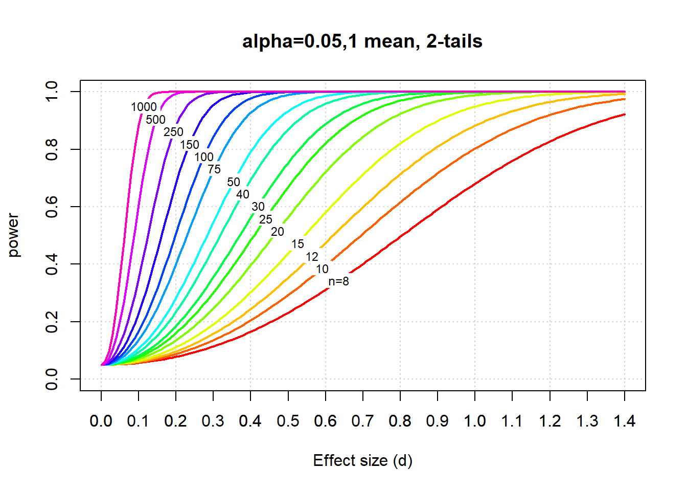
Power curves demonstrate the main things that affect power. First, you can see how power rises from left to right, as we increase the effect size. Second, you can see how power also rises with sample size.
They’re also useful for estimating power without a computer in case your power goes out or something. For example, you can eyeball the curves and guess that if you’d like to design an experiment with a medium effect size of d=0.4 to have a power of 0.8, then you’d need to run about 50 subjects.
Can you see where all the power curves converge when the effect size is zero? That level is a \(\alpha\) = 0.05. This is because when the effect size is zero, the null hypothesis is true, and when the null hypothesis is true, the probability of rejecting \(H_{0}\) is \(\alpha\).
The sets of power curves therefore depend on \(\alpha\). They also depend on whether you are comparing one or two means. A full set of power curves can be found in pdf format at:
9.9 Estimating Power with Simulations
This is one of the most useful things you can do if you switch to a programming language to do your statistics.
Calculating power (the probability of correctly rejecting the null hypothesis) is usually done under very specific violations of the null hypothesis. For example, an independent measures t-test assumes that the population variances are equal and that only the means differ.
However, sometimes it’s useful to calculate power for more complicated violations of the null hypothesis. In these cases there often is not a known distribution to draw p-values from.
A more general way to estimate power is to simulate data repeatedly under some specific assumption about the true distribution and calculate the proportion of times that the null hypothesis is rejected.
Here we’ll do this for a two-tailed t-test.
First we’ll define the population parameters
true.mean <- 100   # true population mean that we'll be sampling from
mu <- 100   # null hypothesis mean (mean we're comparing our sample to)
sigma <- 10  # standard deviation
n <- 10  # sample size
alpha <- .05
The great thing about simulations is that we know the state of the null hypothesis - we can make it true or false and see what happens. We’re starting here with equal means and standard deviations, so \(H_{0}\) is true.
This next chunk of code generates random data sets using rnorm based on the population parameters, runs a t-test on each set, and saves the p-value.
nReps <- 10000  # number of randomly sampled data sets and tests

p.values <- rep(NA,nReps)  # zero-out the vector that will hold the p-values

# start the loop
for (i in 1:nReps) {

  # generate a randomly sampled data set
  x <- rnorm(n,true.mean,sigma)

  # run the hypothesis test
  out <- t.test(x,mu = mu,
                alternative = "two.sided",
                var.equal = F)

  # save the p-value for this iteration
  p.values[i] <- out$p.value
}
All we have to do now is calculate the proportion of times that our simulated p-values are less than \(\alpha\) = 0.05. This is the proportion of times that we’re rejecting \(H_{0}\):
p.sim = sum(p.values<alpha)/nReps

sprintf('We rejected H0 for %g percent of the experiments with alpha = %g',p.sim*100,alpha)
## [1] "We rejected H0 for 4.76 percent of the experiments with alpha = 0.05"Since we set \(H_{0}\) to be true, hopefully this proportion is somewhere around \(\alpha\) = 0.05
Here’s a histogram of the simulated p-values where \(H_{0}\) is true:
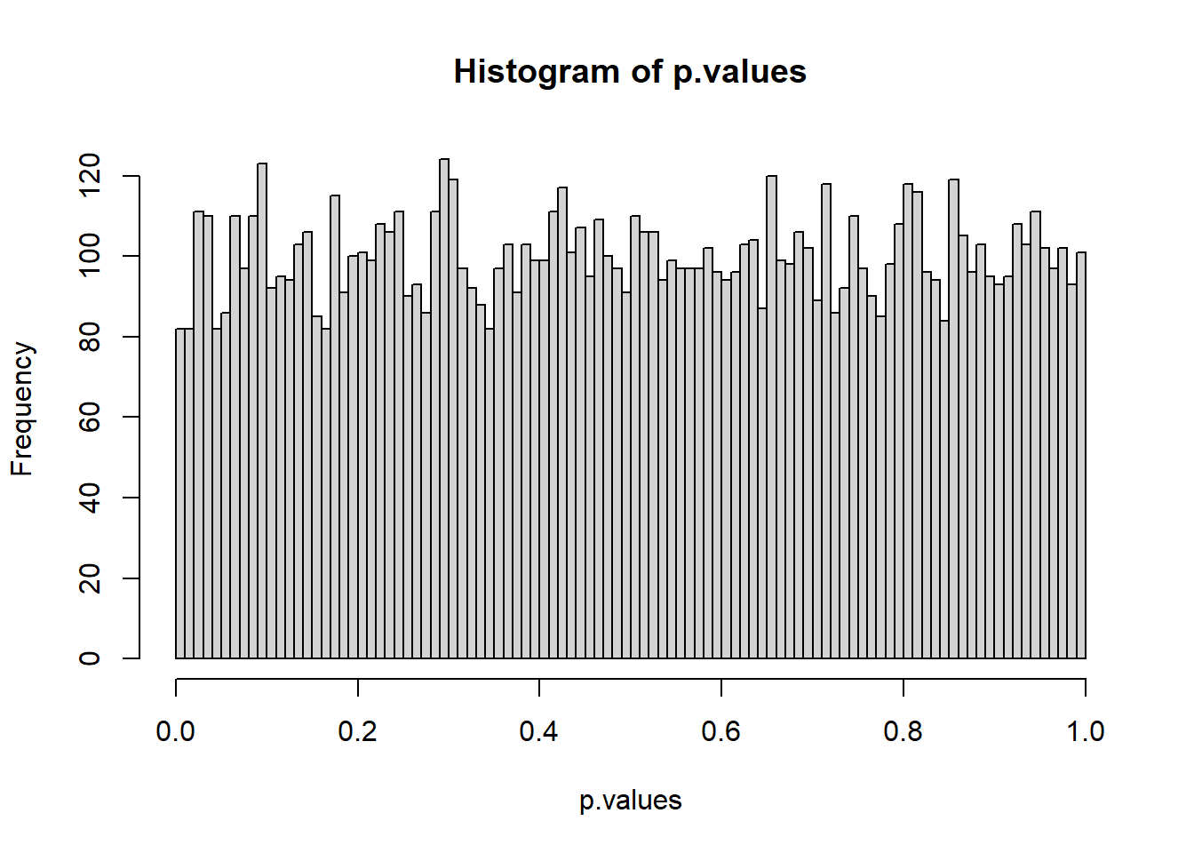
It’s flat! This is important: if \(H_{0}\) is true, then the probability of obtaining any p-value between 0 and 1 is equally likely. It makes sense if you think about it. This is the only distribution for which the proportion of p-values falling below \(\alpha\) is \(\alpha\).
Now lets’ make \(H_{0}\) be false. Here’s the same script but we’ll set mu2 <- 110 instead of 100:
true.mean <- 110   # true population mean that we'll be sampling from
mu <- 100   # null hypothesis mean (mean we're comparing our sample to)
sigma <- 10  # standard deviation
n <- 10  # sample size
alpha <- .05


nReps <- 10000  # number of randomly sampled data sets and tests

p.values <- rep(NA,nReps)  # zero-out the vector that will hold the p-values

# start the loop
for (i in 1:nReps) {

  # generate a randomly sampled data set
  x <- rnorm(n,true.mean,sigma)

  # run the hypothesis test
  out <- t.test(x,mu = mu,
                alternative = "two.sided",
                var.equal = F)

  # save the p-value for this iteration
  p.values[i] <- out$p.value
}
p.sim = sum(p.values<alpha)/nReps

sprintf('We rejected H0 for %g percent of the experiments with alpha = %g',p.sim*100,alpha)
## [1] "We rejected H0 for 80.47 percent of the experiments with alpha = 0.05"Since \(H_{0}\) is false, we’re rejecting more often. You should appreciate that this number, 0.8047 is an estimation of the power of our hypothesis test for this particular violation of \(H_{0}\).
We can compare our estimated power to the value we get from power.t.test. First we have to compute the effect size for our population parameters. We’ll divide the difference between the \(\mu\)s by the calculated pooled standard deviation based on the population \(\sigma\)’s:
# Calculate the effect size
d <-abs(true.mean-mu)/sigma

# Calculate power
out <- power.t.test(n = n,
                   d = d,
                   power = NULL,
                   sig.level =alpha,
                   alternative = "two.sided",
                   strict = T,
                   type ="one.sample" )

# Print out the simulated and calculated powers
sprintf('simulated power: %5.4f',p.sim)
## [1] "simulated power: 0.8047"## [1] "observed power: 0.8031"It’s pretty close! If we increase the size of the simulations we’ll get closer to the results from power.t.test.
Now let’s look at a histogram of the p-values. We’ll get fancy and color the range of the p-values red for when p<0.05
dx <- .01 # class interval width.
# Get the frequency distribution using 'hist'
h <- hist(p.values,
          breaks = seq(0,1,dx),
          plot = FALSE)

# Turn the frequencies into proportions
h$counts <- h$counts/(nReps*dx)

# Create a vector of colors for each bin
colors = rep("red",length(h$breaks))
colors[h$breaks>alpha] <- "green"

# Make a bar graph of proportions using 'colors' so p<alpha is red
plot(h,col=colors,
     ylab ="Proportion",
     main = sprintf('Simulated power: %g\n Calculated power: %g',p.sim,out$power))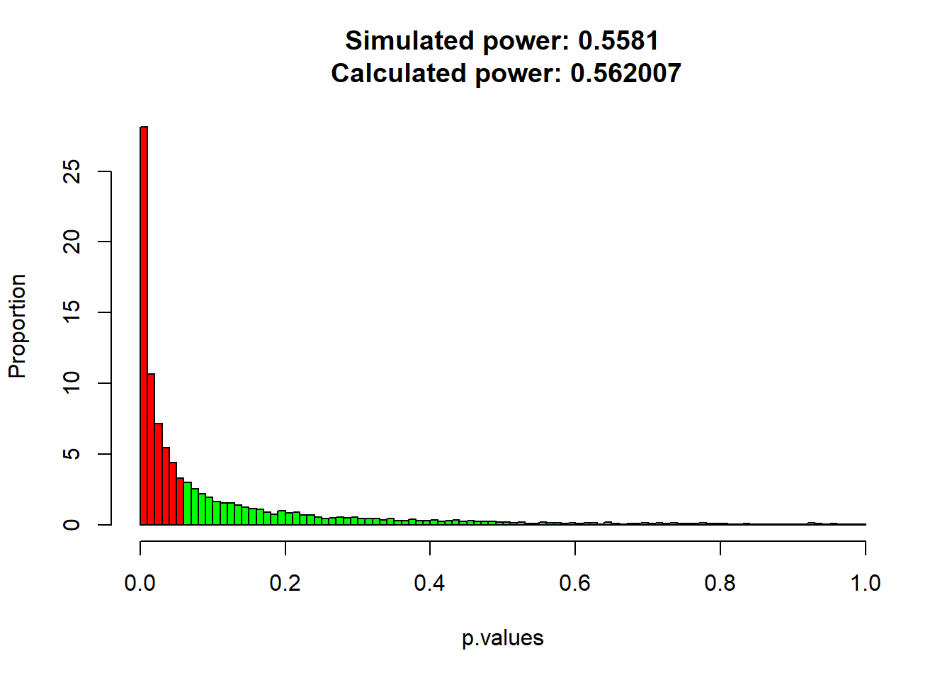
Now the simulated p-values are bunched up to the left. That’s because a higher proportion of p-values are now falling below \(\alpha\).
This distribution of p-values is sometimes called a ‘p-curve’. We’ve learned here that the p-curve is flat when \(H_{0}\) is true, and should bunch up toward small p-values when \(H_{0}\) is false. Finally, the area under the p-curve below \(\alpha\) is the power of our hypothesis test.
You can use the code above to run some interesting simulations. For example, what happens when you keep the population mean the same but change the standard deviation? What happens when you change the sample size?