Chapter 18 Two Factor ANOVA
A two-factor ANOVA is used to test mean differences in a design with two independent variables (factors), called a ‘factorial design’. In a factorial design, observations are collected for every combination of the levels of the two factors. Each combination defines a ‘cell’.
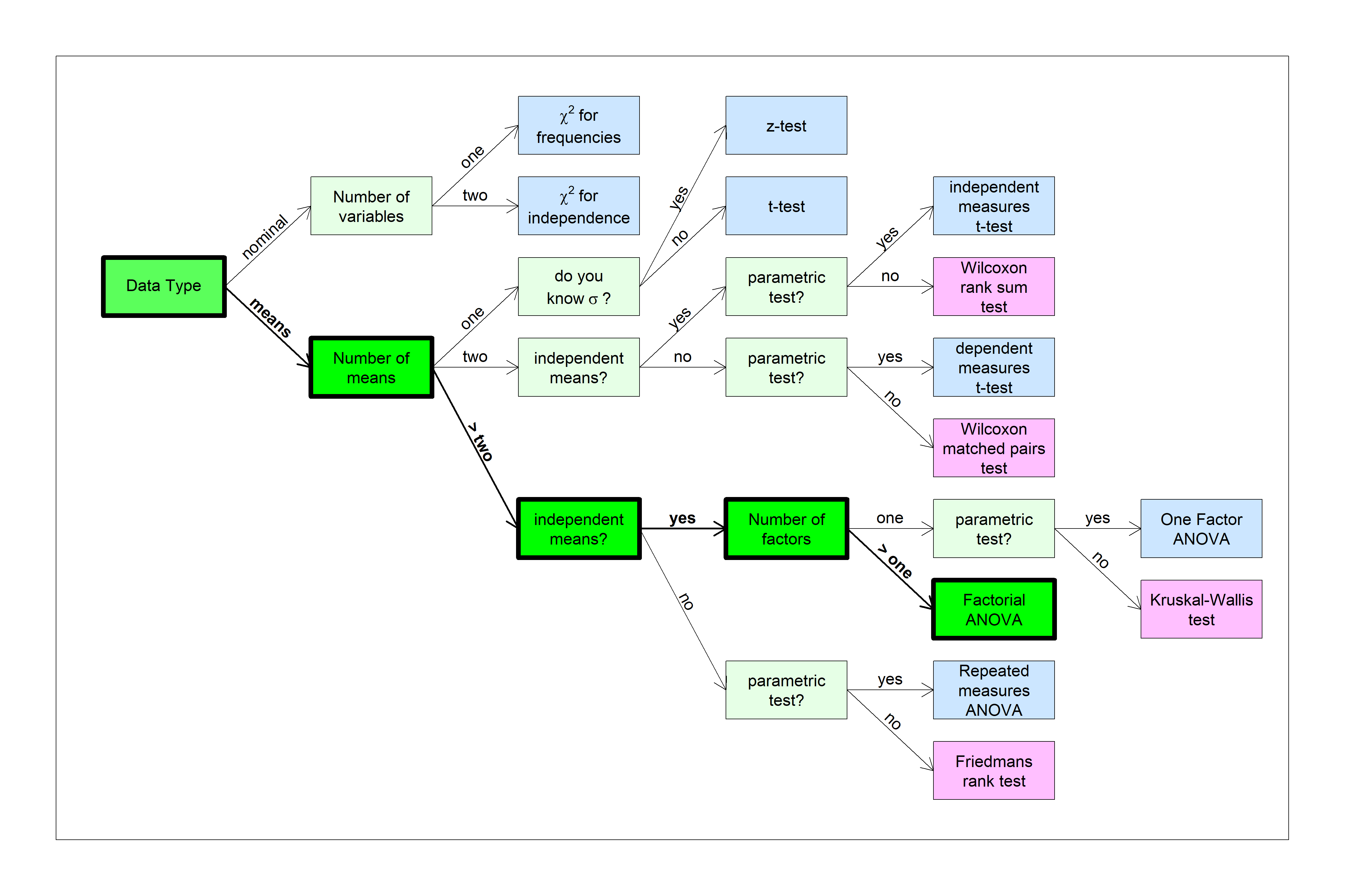
You can find this test in the flow chart here:
We’ll build up to the two-factor ANOVA by starting with a 1-factor ANOVA experiment with contrasts.
18.1 ANOVA Beer and Caffeine Example
Suppose we study the effects of beer and caffeine on response time in a simple reaction-time task. One way to analyze this experiment is to treat it as a one-way ANOVA with four levels:
“no beer, no caffeine” The sober ‘control’ group
“no beer, caffeine” Caffeine only
“beer, no caffeine” Beer only
“beer, caffeine” A fourth group that had both beer and caffeine.
The new aspect of this design is this fourth group. You might just want to compare the effects of either beer or caffeine to the control group, but this fourth group allows to test for something interesting - how the effects of beer and caffeine might interact.
We’ll first treat the data as a one-way ANOVA with three orthogonal contrasts.
To load this existing data from the course website:
data1 <- read.csv('http://courses.washington.edu/psy524a/datasets/BeerCaffeineANOVA1.csv')
# reorder the levels
data1$Condition <- factor(
  data1$Condition,
  levels = c("no beer, no caffeine", "no beer, caffeine",
             "beer, no caffeine",    "beer, caffeine"))
The data is stored in ‘long format’ like this:
| Responsetime | Condition |
|---|---|
| 2.24 | no beer, no caffeine |
| 2.63 | beer, no caffeine |
| 2.27 | beer, no caffeine |
| 1.51 | beer, caffeine |
| 1.84 | no beer, caffeine |
| 2.06 | beer, caffeine |
| 1.39 | no beer, no caffeine |
| 1.94 | beer, no caffeine |
| 2.43 | no beer, no caffeine |
| 1.93 | beer, caffeine |
| 2.68 | beer, caffeine |
| 1.70 | no beer, no caffeine |
| 1.93 | beer, caffeine |
| 0.62 | no beer, caffeine |
| 2.56 | beer, no caffeine |
| 1.65 | beer, caffeine |
| 0.28 | no beer, no caffeine |
| 1.06 | no beer, no caffeine |
| 0.84 | no beer, caffeine |
| 2.07 | beer, no caffeine |
| 1.15 | no beer, no caffeine |
| 2.24 | no beer, no caffeine |
| 2.35 | beer, no caffeine |
| 2.48 | beer, no caffeine |
| 1.72 | no beer, caffeine |
| 1.48 | no beer, no caffeine |
| 1.31 | no beer, caffeine |
| 1.71 | beer, no caffeine |
| 1.63 | no beer, caffeine |
| 1.62 | no beer, no caffeine |
| 1.80 | beer, caffeine |
| 2.19 | beer, no caffeine |
| 1.50 | beer, no caffeine |
| 0.45 | no beer, caffeine |
| 1.53 | no beer, no caffeine |
| 1.37 | beer, caffeine |
| 1.52 | no beer, caffeine |
| 1.35 | beer, caffeine |
| 1.30 | no beer, caffeine |
| 1.75 | no beer, caffeine |
| 2.35 | beer, no caffeine |
| 2.05 | beer, caffeine |
| 2.69 | no beer, no caffeine |
| 1.91 | no beer, caffeine |
| 2.68 | beer, caffeine |
| 1.33 | no beer, caffeine |
| 2.47 | beer, no caffeine |
| 1.29 | beer, caffeine |
Here are the summary statistics from this data set:
The four conditions, or ‘levels’ are “no beer, no caffeine”, “no beer, caffeine”, “beer, no caffeine”, and “beer, caffeine”
| mean | n | sd | sem | |
|---|---|---|---|---|
| no beer, no caffeine | 1.650833 | 12 | 0.6725455 | 0.1941472 |
| no beer, caffeine | 1.351667 | 12 | 0.4829235 | 0.1394080 |
| beer, no caffeine | 2.210000 | 12 | 0.3476153 | 0.1003479 |
| beer, caffeine | 1.858333 | 12 | 0.4696194 | 0.1355675 |
Here’s a plot of the means with error bars as the standard error of the mean:

It looks like the means do differ from one another. To check, here’s the result of the omnibus ANOVA:
## Analysis of Variance Table
##
## Response: Responsetime
##           Df Sum Sq Mean Sq F value   Pr(>F)
## Condition  3  4.687 1.56234  6.0856 0.001478 **
## Residuals 44 11.296 0.25673
## ---
## Signif. codes:  0 '***' 0.001 '**' 0.01 '*' 0.05 '.' 0.1 ' ' 1
This shows that some combination of beer and caffeine have a significant effect on response times.
Let’s look at the effects of beer and ceffeine on reaction times separately.
18.2 Effect of Beer
We could run a t-test comparing the “beer, no caffeine” group to the “no beer, no caffeine” group, but in a factorial design we can use the full set of data and calculate the effect of beer after averaging across the two levels of caffeine. Averaging across the other condition produces what’s called the ‘main effect’ of beer, and can be done with a contrast with these weights:
| no beer, no caffeine | no beer, caffeine | beer, no caffeine | beer, caffeine | |
|---|---|---|---|---|
| Effect of Beer | 1 | 1 | -1 | -1 |
Just as we did in the last chapter, we first run emmeans on the output of `lm’ which will be used for all of our contrasts:
Then for the main effect of beer:
##  contrast        estimate    SE df t.ratio p.value
##  c(1, 1, -1, -1)    -1.07 0.293 44  -3.643  0.0007
There is a significant effect of beer on response times. Since we’re subtracting the beer from the without beer conditions, our negative value of ‘estimate’ (\(\psi\)) means that the responses times for beer are greater than for no beer. Beer increases response times.
18.3 Effect of Caffeine
This contrast averages across beer conditions and tests for the main effect of caffeine on response times.
| no beer, no caffeine | no beer, caffeine | beer, no caffeine | beer, caffeine | |
|---|---|---|---|---|
| Effect of Caffeine | 1 | -1 | 1 | -1 |
##  contrast        estimate    SE df t.ratio p.value
##  c(1, -1, 1, -1)    0.651 0.293 44   2.225  0.0313
Caffeine has a significant effect on response times - this time \(\psi\) is positive, so response times with caffeine are faster than for without caffeine. Caffeine reduces response times.
18.4 The Third Contrast: Interaction
For four levels or groups, there are three independent contrast. Here’s the third contrast:
| no beer, no caffeine | no beer, caffeine | beer, no caffeine | beer, caffeine | |
|---|---|---|---|---|
| Beer X Caffeine | -1 | 1 | 1 | -1 |
What does that third contrast measure? Symbolically, the contrast combines the conditions as:
-[no beer, no caffeine] + [no beer, caffeine] + [beer, no caffeine] - [beer, caffeine]
Rearranging the terms as a difference of differences:
([beer, no caffeine] - [no beer, no caffeine]) - ([beer, caffeine]-[no beer, caffeine])
The first difference is the effect of beer without caffeine. The second difference is the effect of beer with caffeine. The difference of the differences is a measure of how the effect of beer changes by adding caffeine. In statistical terms, we call this the interaction between the effects of beer and caffeine on response times. Interactions are labeled with an ‘X’, so this contrast is labeled as ‘Beer X Caffeine’.
You might have noticed the parallel between this and the \(\chi^{2}\) test of independence. This is the same concept, but for means rather than frequencies.
The results of the F-tests for this third contrast is:
##  contrast        estimate    SE df t.ratio p.value
##  c(-1, 1, 1, -1)   0.0525 0.293 44   0.179  0.8584
We fail to reject \(H_{0}\), so there is no significant interaction between the effects of beer and caffeine on response times. This means that adding beer increases response times effectively the same amount regardless of caffeine. Conversely, caffeine reduces response times effectively the same amount with or without beer. Notice the use of the word ‘effectively’ here. We should be careful about saying that ‘beer increases response times the same amount, regardless of caffeine’ because this isn’t true. There is a slight numerical difference, but it is not statistically significant.
18.5 Partitioning \(SS_{between}\)
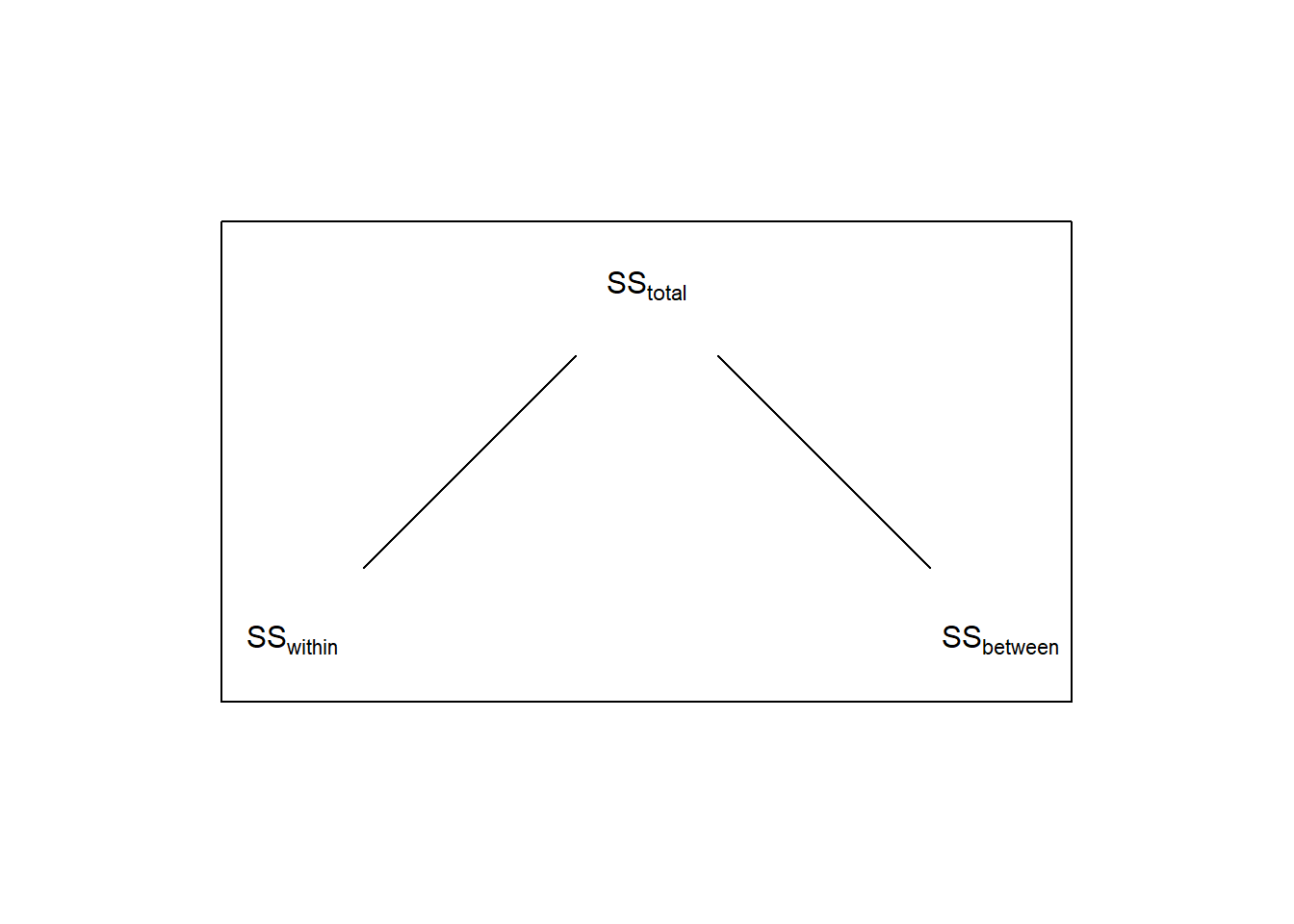
Recall that for a 1-factor ANOVA, \(SS_{total}\) is broken down in to two parts \(SS_{within}\) and \(SS_{between}\).
In the chapter section on APriori and post-hoc tests we discussed how the sums of squared for independent contrasts is a way of breaking down the total variability between the means, \(SS_{between}\). The same is true here for our three orthogonal contrasts. From the last chapter we showed that if you consider the contrasts as F-tests:
\[SS_{contrast} = t^2MS_{within}\]
We can use R to calculate \(SS_contrast\) by taking \(MS_within\) from the ANOVA:
# run the omnibus ANOVA and take out SS_between and MS_within
anova1.out <- anova(lm1.out)
round(anova1.out,2)
## Analysis of Variance Table
##
## Response: Responsetime
## Df Sum Sq Mean Sq F value Pr(>F)
## Condition 3 4.69 1.56 6.09 < 2.2e-16 ***
## Residuals 44 11.30 0.26
## ---
## Signif. codes: 0 '***' 0.001 '**' 0.01 '*' 0.05 '.' 0.1 ' ' 1And then run all three contrasts together and calcuate \(SS_{contrast}\):
contrasts <- list(beer = c(1,1,-1,-1),
                  caffeine = c(1,-1,1,-1),
                  interaction = c(1, -1, -1, 1))
contrast.result <- summary(contrast(emm1, method = contrasts))
# Calculate SS_contrast = (t^2)(MS_contrast) and append it to contrast.result
contrast.result$SS_contrast <- round(contrast.result$t.ratio^2*MS_within,2)
contrast.result
## contrast estimate SE df t.ratio p.value SS_contrast
## beer -1.0658 0.293 44 -3.643 0.0007 3.41
## caffeine 0.6508 0.293 44 2.225 0.0313 1.27
## interaction -0.0525 0.293 44 -0.179 0.8584 0.01Like the last chapter, you can see how \(SS_{between}\) is divided up among the three contrasts. Summing up the three \(SS_{contrast}\) values gives us \(SS_{between}\):
\[\sum{SS_{contrast}} = 3.41+1.27+0.01 = 4.69 = SS_{between}\]
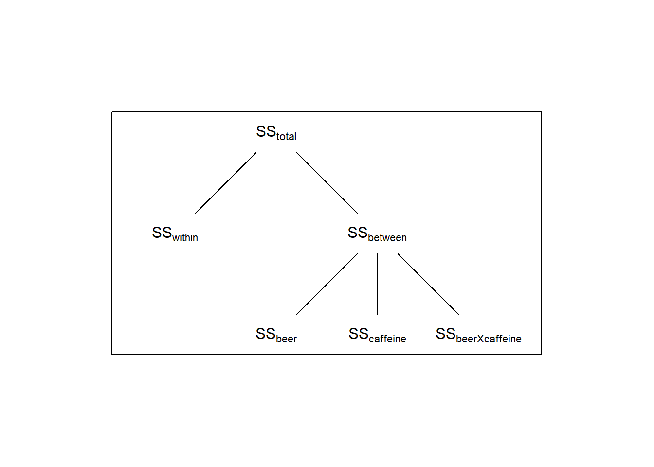
The three contrasts have partitioned the total variability between the four means into three separate independent tests - each telling us something different about what is driving the significance of the ‘omnibus’ F-test. If we call the sums-of-squares for each of the three contrasts \(SS_{beer}\), \(SS_{caffeine}\), and \(SS_{beerXcaffeine}\) (where the ‘\(X\)’ means ’interaction), we can expand the above diagram to this:
This example is a ‘balanced’ factdorial design, which means that the sample sizes are the same for all conditions.
A standard way to analyze a factorial design is to break the overall variability between the means into separate hypothesis tests - a main effect for each factor, and their interactions. In this next section we’ll show how treating the same data that we just discussed as a 2-factor ANOVA gives us the exact same result as treating the same results as a 1-factor ANOVA with three contrasts.
18.6 2-Factor ANOVA
I’ve saved the same data set but in a way that’s ready to be analyzed as a factorial design experiment. We’ll load it in here:
data2 <- read.csv('http://courses.washington.edu/psy524a/datasets/BeerCaffeineANOVA2.csv')
# order the levels for the two factors (alphabetical by default)
data2$caffeine <- factor(data2$caffeine,levels = c('no caffeine','caffeine'))
data2$beer <- factor(data2$beer,levels = c('no beer','beer'))
The data is stored in ‘long format’ like this:
| Responsetime | caffeine | beer |
|---|---|---|
| 2.24 | no caffeine | no beer |
| 1.62 | no caffeine | no beer |
| 1.48 | no caffeine | no beer |
| 1.70 | no caffeine | no beer |
| 1.06 | no caffeine | no beer |
| 1.39 | no caffeine | no beer |
| 2.69 | no caffeine | no beer |
| 0.28 | no caffeine | no beer |
| 2.24 | no caffeine | no beer |
| 1.15 | no caffeine | no beer |
| 1.53 | no caffeine | no beer |
| 2.43 | no caffeine | no beer |
| 1.71 | no caffeine | beer |
| 2.19 | no caffeine | beer |
| 2.27 | no caffeine | beer |
| 2.35 | no caffeine | beer |
| 2.47 | no caffeine | beer |
| 2.07 | no caffeine | beer |
| 2.56 | no caffeine | beer |
| 2.35 | no caffeine | beer |
| 1.50 | no caffeine | beer |
| 2.63 | no caffeine | beer |
| 2.48 | no caffeine | beer |
| 1.94 | no caffeine | beer |
| 0.62 | caffeine | no beer |
| 1.72 | caffeine | no beer |
| 1.75 | caffeine | no beer |
| 1.84 | caffeine | no beer |
| 1.30 | caffeine | no beer |
| 1.52 | caffeine | no beer |
| 1.31 | caffeine | no beer |
| 1.63 | caffeine | no beer |
| 1.91 | caffeine | no beer |
| 1.33 | caffeine | no beer |
| 0.84 | caffeine | no beer |
| 0.45 | caffeine | no beer |
| 2.05 | caffeine | beer |
| 1.51 | caffeine | beer |
| 1.65 | caffeine | beer |
| 2.68 | caffeine | beer |
| 2.06 | caffeine | beer |
| 1.80 | caffeine | beer |
| 2.68 | caffeine | beer |
| 1.93 | caffeine | beer |
| 1.29 | caffeine | beer |
| 1.93 | caffeine | beer |
| 1.35 | caffeine | beer |
| 1.37 | caffeine | beer |
The data format has the same ‘ResponseTime’ column, but now it has two columns instead of one that define the two factors. The ‘caffeine’ column has two levels: ‘caffeine’ and ‘no caffeine’. Similarly the ‘beer’ column has two levels ‘beer’ and ‘no beer’. This way of storing the data is called ‘long format’, where which each row corresponds to a single observation.
This experiment is called a 2x2 factorial design because each of the two factors has two levels. We can summarize the results in the form of matrices with rows and columns corresponding to the two factors. We’ll set the ‘row factor’ as ‘caffeine’ and the ‘column factor’ as ‘beer’. That is, ‘beer’ varies across the rows and ‘caffeine’ varies across the column. Here’s the 2x2 table for the means:
| no beer | beer | |
|---|---|---|
| no caffeine | 1.6508 | 2.2100 |
| caffeine | 1.3517 | 1.8583 |
Instead of bar graphs, it’s common to plot results of factorial designs as data points with lines connecting them. By default, I plot the column factor along the x-axis and define the row factor in the legend. There are various ways of doing this with R. Here’s an example for our data. It requires both ‘ggplot2’ and the ‘dplyr’ libraries. Both are part of the ‘tidyverse’ package.
# Do this to avoid an annoying error message
options(dplyr.summarise.inform = FALSE)
# Make a table (tibble) with generic names
summary.table <- data2 %>%
  dplyr::group_by(caffeine,beer) %>%
  dplyr::summarise(
    m = mean(Responsetime),
    sem = sd(Responsetime)/sqrt(length(Responsetime))
  )
  # plot with error bars, replacing generic names with specific names
  ggplot(summary.table, aes(beer, m)) +
    geom_errorbar(
      aes(ymin = m-sem, ymax = m+sem, color = caffeine),
      position = position_dodge(0), width = 0.5)+
    geom_line(aes(group = caffeine,color = caffeine)) +
    geom_point(aes(group = caffeine,color = caffeine),size = 5) +
    scale_color_manual(values = rainbow(2)) +
    xlab('beer') +
    ylab('Response Time (s)') +
    theme_bw()
18.7 Within-Cell Variance (\(MS_{wc}\))
All three F-tests for a 2-factor ANOVA will use the same value in the denominator, \(MS_{wc}\), which is the within-cell mean-squared error. We start with calculating \(SS_{wc}\) which is, like the 1-factor ANOVA, the sums of squared deviation of each score from the mean of the cell that it came from:
\[SS_{wc} = \sum_i{\sum_j{\sum_k{(X_{ijk}-\overline{X}_{ij})^2}}}\] Where \(X_{ijk}\) is the k’th score in the group \(i,j\) that has level i for the first factor and j for the second factor. \(\overline{X}_{ij}\) is the mean of the scores in group \(i,j\).
The sums of squares for each condition is:
| no beer | beer | |
|---|---|---|
| no caffeine | 4.9755 | 1.3292 |
| caffeine | 2.5654 | 2.4260 |
\(SS_{wc}\) is the sum of these individual within-cell sums of squares:
\[SS_{wc} = 4.9755+2.5654+1.3292+2.426 = 11.2961\]
Each cell contributes n-1 degrees of freedom to \(SS_{wc}\), so the degrees of freedom for all cells is N-k, where k is the total number of cells and N is the total sample size (n \(\times\) k):
\[df_{wc} = 48 - 4 = 44\]
Mean-squared error is, as always, \(\frac{SS}{df}\):
\[MS_{wc} = \frac{SS_{wc}}{df_{wc}} = \frac{11.296}{44} = 0.2567\]
This is the same \(MS\) value and df as \(MS_{w}\) from above when we treated the same data as a 1-factor ANOVA design.
The three contrasts that we used for the 1-factor ANOVA example correspond to what we call ‘main effects’ for the factors and the ‘interaction’ between the factors. To calculate the main effects by hand we need to calculate the means across the rows and columns of our factors. Here’s a table with the row and sum means in the ‘margins’:
| no beer | beer | means | |
|---|---|---|---|
| no caffeine | 1.6508 | 2.2100 | 1.9304 |
| caffeine | 1.3517 | 1.8583 | 1.6050 |
| means | 1.5012 | 2.0342 | 1.7677 |
The bottom-right number is the mean of the means, which is the grand mean (\(\overline{\overline{X}}\) = 1.7677)
18.7.1 Main Effect for Columns (Beer)
Calculating main effects is lot like calculating \(SS_{between}\) for the 1-factor ANOVA. For the main effect for columns, we calculate the sums of squared deviations of the column means from the grand mean, and scale it by the number of samples that contributed to each column mean. For our example, the sums of square deviations is:
\[(1.5012-1.7677)^2+(2.0342-1.7677)^2=0.071+0.071 = 0.142\]
There are \(2 \times 12 = 24\) samples for each column mean, so the sums of squared for the columns, called \(SS_{C}\) is
\[SS_{C} = (24)(0.142) = 3.408\]
Since 2 means contributing to \(SS_{R}\), so the degrees of freedom is \(df_{R}\) = 2 -1 = 1
\(MS_{C}\) is therefore
\[\frac{SS_{C}}{df_{C}} = \frac{3.4080}{1} = 3.4080\]
The F-statistic for this main effect is \(MS_{C}\) divided by our common denominator, \(MS_{wc}\)
\[F = \frac{MS_{C}}{MS_{wc}} = \frac{3.4080}{0.2567} = 13.2748\]
We can calculate the p-value for this main effect using pf:
## [1] 0.0007060154Notice that the F and p-values are the same as for the first contrast in the 1-way ANOVA above. If you work out the algebra you’ll find that the math is the same. The main effect in a multi-factorial ANOVA is exactly the same as the appropriate contrast in a 1-factor ANOVA.
18.7.2 Main Effect for Rows (Caffeine)
The calculations for finding the main effect of rows (Caffeine) on response times is completely analogous to finding the main effect for columns. We use our row means in the table above, which are the averages across the two beer conditions.
The sums of squared deviations for the means for rows is:
\[(1.9304-1.7677)^2+(1.605-1.7677)^2=0.0265+0.0265 = 0.053\]
There are \(2 \times 12 = 24\) samples for each row mean, so the sums of squared for the row, called \(SS_{R}\) is
\[SS_{R} = (24)(0.0529) = 1.2708\]
There are 2 means contributing to \(SS_{R}\), so the degrees of freedom is \(df_{R}\) = 2 -1 = 1
\(MS_{R}\) is therefore
\[\frac{SS_{R}}{df_{R}} = \frac{1.2708}{1} = 1.2708\]
The F-statistic for this main effect is \(MS_{R}\) divided by our common denominator, \(MS_{wc}\)
\[F = \frac{MS_{R}}{MS_{wc}} = \frac{1.2708}{0.2567} = 4.9498\]
The p-value for the main effect of Beer is:
## [1] 0.0312691418.7.3 Interaction Between Beer and Caffeine
The third contrast in the 1-factor ANOVA measured the differential effect of caffeine on response times across the two beer conditions (or vice versa). Recall that for a 1-factor ANOVA the sums of squares associated with three orthogonal conditions adds up to \(SS_{between}\) for four groups. Also, recall that \(SS_{between} + SS_{within} = SS_{total}\).
The easiest way to calculate the sums of square value for interaction is to appreciate that
\[SS_{total} = SS_{caffeine} + SS_{beer} + SS_{caffeineXbeer} + SS_{wc}\]
The total sums of squares is \(SS_{total}\) = 15.983.
Therefore,
\[SS_{caffeineXbeer} = SS_{total} - (SS_{wc} + SS_{caffeine} + SS_{beer})\]
so
\[SS_{RXC} = SS_{total}-SS_{R}-SS_{C}-SS_{wc} = 15.9830 - 1.2708 - 3.4080 - 11.2960 = 0.0083\]
The degrees of freedom for this interaction term is (\(n_{rows}\)-1)*(\(n_{cols}\)-1):
\[df_{RXC} = (n_{rows}-1)(n_{cols}-1) = (2-1)(2-1) = 1\]
So the mean-squared error for the interaction is
\[\frac{SS_{RXC}}{df_{RXC}} = \frac{0.0083}{1} = 0.0083\]
Using \(SS_{wc}\) for the denominator again, the F-statistic is:
$$
The p-value for the interaction is:
## [1] 0.8584132There is not a significant interaction between caffeine and beer on response times. Compare these numbers to the results of the third contrast in the 1-factor ANOVA above.
We typically summarize our calculations and results in a table like this:
| df | SS | MS | F | p | |
|---|---|---|---|---|---|
| caffeine | 1 | 1.2708 | 1.2708 | 4.9498 | p = 0.0313 |
| beer | 1 | 3.4080 | 3.408 | 13.2748 | p = 0.0007 |
| interaction | 1 | 0.0083 | 0.0083 | 0.0322 | p = 0.8584 |
| wc | 44 | 11.2960 | 0.2567 | ||
| Total | 47 | 15.9830 |
Using APA format we state, for our three tests:
There is a main effect of caffeine. F(1,44) = 4.9498, p = 0.0313.
There is a main effect of beer. F(1,44) = 13.2748, p = 0.0007.
There is not a significant interaction between caffeine and beer. F(1,44) = 0.0322, p = 0.8584.
You might have noticed that didn’t use any correction for familywise error for these three tests. There is a general consensus that the main effects and the interaction do not require familywise error correction. But if we treat the same data as a 1-factor design with three planned contrasts, we should apply error correction (like Bonferroni) even though the math and p-values are the same. If you find discrepancies like this baffling you are not alone.
18.8 The two-factor ANOVA with R
Conducting a two-factor ANOVA with R is a lot like for 1-factor ANOVA. We’ll use the lm function and pass it through the anova function to get our table and statistics. The difference is the definition of the formula. Here we’ll use: Responsetime ~ caffieene*beer. The use of ’*’ is the way to ask lm to predict response times with not only the main effects of caffeine and beer but also their interaction:
## Analysis of Variance Table
##
## Response: Responsetime
##               Df  Sum Sq Mean Sq F value   Pr(>F)
## caffeine       1  1.2708  1.2708  4.9498 0.031269 *
## beer           1  3.4080  3.4080 13.2748 0.000706 ***
## caffeine:beer  1  0.0083  0.0083  0.0322 0.858395
## Residuals     44 11.2960  0.2567
## ---
## Signif. codes:  0 '***' 0.001 '**' 0.01 '*' 0.05 '.' 0.1 ' ' 1
All of these numbers should look familiar.
18.9 A 2x3 Factorial Example
Factorial designs let you study the effects of one factor across multiple levels of another factor (or factors). In this made-up example, we’ll study the effect of two kinds of diets: “Atkins” and “pea soup” on the systolic blood pressure (BP, in mm Hg) for three exercise levels: “none”, “a little”, and “a lot”. A systolic blood pressure less than 120 mm Hg is considered normal. 20 subjects participated in each of the 2x3 = 6 groups for a total of 120 subjects. Here’s how to load in the data from the course website and order the levels:
data3 <- read.csv('http://courses.washington.edu/psy524a/datasets/DietExerciseBP.csv')
data3$Diet <- factor(data3$Diet,levels = c('Atkins','pea soup'))
data3$Exercise <- factor(data3$Exercise,levels = c('none','a little','a lot'))
The data is stored in ‘long format’ like this:
| BP | Diet | Exercise |
|---|---|---|
| 125.6032 | Atkins | none |
| 137.7546 | Atkins | none |
| 122.4656 | Atkins | none |
| 158.9292 | Atkins | none |
| 139.9426 | Atkins | none |
| 122.6930 | Atkins | none |
| 142.3114 | Atkins | none |
| 146.0749 | Atkins | none |
| 143.6367 | Atkins | none |
| 130.4192 | Atkins | none |
| 157.6767 | Atkins | none |
| 140.8476 | Atkins | none |
| 125.6814 | Atkins | none |
| 101.7795 | Atkins | none |
| 151.8740 | Atkins | none |
| 134.3260 | Atkins | none |
| 134.7571 | Atkins | none |
| 149.1575 | Atkins | none |
| 147.3183 | Atkins | none |
| 143.9085 | Atkins | none |
| 148.7847 | Atkins | a little |
| 146.7320 | Atkins | a little |
| 136.1185 | Atkins | a little |
| 105.1597 | Atkins | a little |
| 144.2974 | Atkins | a little |
| 134.1581 | Atkins | a little |
| 132.6631 | Atkins | a little |
| 112.9387 | Atkins | a little |
| 127.8277 | Atkins | a little |
| 141.2691 | Atkins | a little |
| 155.3802 | Atkins | a little |
| 133.4582 | Atkins | a little |
| 140.8151 | Atkins | a little |
| 134.1929 | Atkins | a little |
| 114.3441 | Atkins | a little |
| 128.7751 | Atkins | a little |
| 129.0857 | Atkins | a little |
| 134.1103 | Atkins | a little |
| 151.5004 | Atkins | a little |
| 146.4476 | Atkins | a little |
| 132.5321 | Atkins | a lot |
| 131.1996 | Atkins | a lot |
| 145.4545 | Atkins | a lot |
| 143.3499 | Atkins | a lot |
| 124.6687 | Atkins | a lot |
| 124.3876 | Atkins | a lot |
| 140.4687 | Atkins | a lot |
| 146.5280 | Atkins | a lot |
| 133.3148 | Atkins | a lot |
| 148.2166 | Atkins | a lot |
| 140.9716 | Atkins | a lot |
| 125.8196 | Atkins | a lot |
| 140.1168 | Atkins | a lot |
| 118.0596 | Atkins | a lot |
| 156.4954 | Atkins | a lot |
| 164.7060 | Atkins | a lot |
| 129.4917 | Atkins | a lot |
| 119.3380 | Atkins | a lot |
| 143.5458 | Atkins | a lot |
| 132.9742 | Atkins | a lot |
| 171.0243 | pea soup | none |
| 134.4114 | pea soup | none |
| 145.3461 | pea soup | none |
| 135.4200 | pea soup | none |
| 123.8509 | pea soup | none |
| 137.8319 | pea soup | none |
| 107.9256 | pea soup | none |
| 156.9833 | pea soup | none |
| 137.2988 | pea soup | none |
| 167.5892 | pea soup | none |
| 142.1326 | pea soup | none |
| 124.3508 | pea soup | none |
| 144.1609 | pea soup | none |
| 120.9885 | pea soup | none |
| 116.1955 | pea soup | none |
| 139.3717 | pea soup | none |
| 128.3506 | pea soup | none |
| 135.0166 | pea soup | none |
| 136.1151 | pea soup | none |
| 126.1572 | pea soup | none |
| 121.4700 | pea soup | a little |
| 127.9723 | pea soup | a little |
| 147.6713 | pea soup | a little |
| 107.1465 | pea soup | a little |
| 138.9092 | pea soup | a little |
| 134.9943 | pea soup | a little |
| 145.9465 | pea soup | a little |
| 125.4372 | pea soup | a little |
| 135.5503 | pea soup | a little |
| 134.0065 | pea soup | a little |
| 121.8622 | pea soup | a little |
| 148.1180 | pea soup | a little |
| 147.4060 | pea soup | a little |
| 140.5032 | pea soup | a little |
| 153.8025 | pea soup | a little |
| 138.3773 | pea soup | a little |
| 110.8511 | pea soup | a little |
| 121.4010 | pea soup | a little |
| 111.6308 | pea soup | a little |
| 122.8990 | pea soup | a little |
| 110.6945 | pea soup | a lot |
| 120.6317 | pea soup | a lot |
| 106.3362 | pea soup | a lot |
| 122.3704 | pea soup | a lot |
| 110.1812 | pea soup | a lot |
| 146.5093 | pea soup | a lot |
| 130.7506 | pea soup | a lot |
| 133.6526 | pea soup | a lot |
| 125.7628 | pea soup | a lot |
| 145.2326 | pea soup | a lot |
| 110.4640 | pea soup | a lot |
| 113.0753 | pea soup | a lot |
| 141.4842 | pea soup | a lot |
| 110.2396 | pea soup | a lot |
| 116.8893 | pea soup | a lot |
| 114.1079 | pea soup | a lot |
| 115.2001 | pea soup | a lot |
| 115.8133 | pea soup | a lot |
| 127.4128 | pea soup | a lot |
| 117.3400 | pea soup | a lot |
Here’s a plot of the means with error bars:
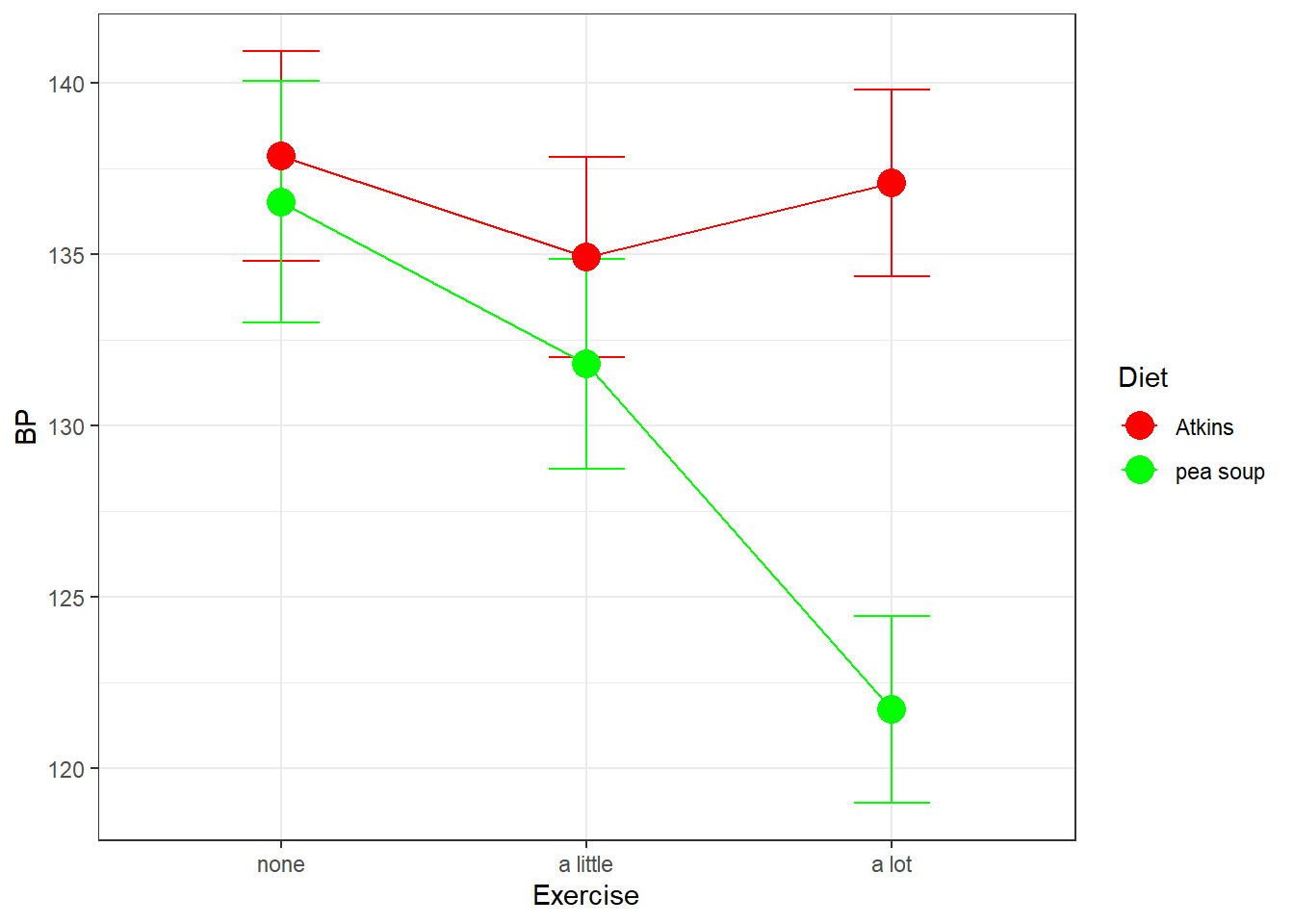
Here we’ve defined the row factor to be Diet and the column factor to be Exercise.
From the graph it looks like the Atkins diet has little effect on systolic blood pressure across exercise levels, but the pea soup diet does seem to lead to lower BP for higher levels of exercise.
The math behind running a 2-factor ANOVA on this design is the same as for the 2x2 example above. We’ll skip all of the details and jump straight to running the ANOVA with R.
The syntax for running the ANOVA is to define the model as BP ~ Diet*Exercise, which is asking lm to predict BP by a combination of Diet, Exercise, and the interaction between Diet and Exercise.
This will be done in two steps, saving the output of lm to be used later.
## Analysis of Variance Table
##
## Response: BP
##                Df  Sum Sq Mean Sq F value   Pr(>F)
## Diet            1  1308.3 1308.32  7.2015 0.008369 **
## Exercise        2  1216.0  608.02  3.3468 0.038689 *
## Diet:Exercise   2  1169.6  584.80  3.2190 0.043658 *
## Residuals     114 20710.7  181.67
## ---
## Signif. codes:  0 '***' 0.001 '**' 0.01 '*' 0.05 '.' 0.1 ' ' 1
Using APA format we’d say:
There is a main effect of Diet. F(1,114) = 7.2015, p = 0.0084.
There is a main effect of Exercise. F(2,114) = 3.3468, p = 0.0387.
There is a significant interaction between Diet and Exercise. F(2,114) = 3.2190, p = 0.0437.
All three hypothesis tests are statistically significant, but this doesn’t really tell us much about what’s driving the effects of Diet and Exercise on BP. As discussed above when we plotted the results, what seems to be happening is that only the subjects on the pea soup diet are influenced by Exercise.
It might make sense, instead, to run two ANOVAs on the data, one for the Atkins diet and one for the pea soup diet. We expect to find that most of variability across the means is driven by the effect of Exercise for the pea soup dieters.
18.10 Simple Effects
Running ANOVAs on subsets of the data like this is called a simple effects analysis. Running separate ANOVAs on each level of Diet is studying the simple effects of Exercise by Diet. I remember this by replacing the word ‘by’ with ‘for every level of’. That is, this simple effect analysis is studying the effect of Exercise on BP for every level of Diet.
Running simple effects is the same as running separate ANOVA’s for each level of Diet, except that we borrow the \(MS_{wc}\) value from the original 2-factor ANOVA. We’ll do this by hand first, and then with R’s joint_test function from the emmeans package. We can use the subset function to pull out the data for each of the two diets”:
# Atkins diet:
anova3.out.Atkins <- anova(lm(BP ~ Exercise,data = subset(data3,Diet == 'Atkins') ))
anova3.out.Atkins
## Analysis of Variance Table
##
## Response: BP
## Df Sum Sq Mean Sq F value Pr(>F)
## Exercise 2 93.9 46.939 0.2783 0.7581
## Residuals 57 9614.3 168.672# pea soup diet:
anova3.out.peasoup <- anova(lm(BP ~ Exercise,data = subset(data3,Diet == 'pea soup') ))
anova3.out.peasoup## Analysis of Variance Table
##
## Response: BP
## Df Sum Sq Mean Sq F value Pr(>F)
## Exercise 2 2291.8 1145.88 5.8862 0.004744 **
## Residuals 57 11096.4 194.67
## ---
## Signif. codes: 0 '***' 0.001 '**' 0.01 '*' 0.05 '.' 0.1 ' ' 1If we assume homogeneity of variance, then we can replace the denominator of these F-tests with the denominator of the two-factor ANOVA, \(MS_{wc}\) = 181.6727. Since \(MS_{wc}\) is based on the entire data set, it be a better estimate of the population variance. It also has a larger df which helps with power.
To do this by hand we need to pull out \(MS_{wc}\) from the output from the original two factor ANOVA and recalculate our F-statistics and p-values using pf:
# from the 2-factor ANOVA, MS_wc is the fourth mean squared in the list
MS_wc <- anova3.out$`Mean Sq`[4]
df_wc <- anova3.out$Df[4]

# Atkins
MS_Atkins <- anova3.out.Atkins$`Mean Sq`[1]
df_Atkins <- anova3.out.Atkins$Df[1]
F_Atkins <- MS_Atkins/MS_wc
p_Atkins <- 1-pf(F_Atkins,df_Atkins,df_wc)

# pea soup
MS_peasoup <- anova3.out.peasoup$`Mean Sq`[1]
df_peasoup <- anova3.out.peasoup$Df[1]
F_peasoup <- MS_peasoup/MS_wc
p_peasoup <- 1-pf(F_peasoup,df_peasoup,df_wc)

sprintf('Atkins:    F(%d,%d)= %5.4f,p = %5.6f',df_Atkins,df_wc,F_Atkins,p_Atkins)
## [1] "Atkins: F(2,114)= 0.2584,p = 0.772759"## [1] "pea soup: F(2,114)= 6.3074,p = 0.002523"The p-values didn’t change much when substituting \(MS_{wc}\), but every little bit of power helps.
18.10.1 Simple effects with R
The package emmeans provides the function joint_tests which is an easy way to run simple effects. It uses the output of ‘lm’ used above in the two-factor ANOVA. This produces the same results as what we did by hand above:
## Diet = Atkins:
##  model term df1 df2 F.ratio p.value
##  Exercise     2 114   0.258  0.7728
##
## Diet = pea soup:
##  model term df1 df2 F.ratio p.value
##  Exercise     2 114   6.307  0.0025
18.11 Additivity of Simple Effects
These two simple effects have an interesting relation with the three tests from the original 2-factor ANOVA. It turns out that the SS associated with these two simple effects add up the SS associated with the main effects of Exercise plus the SS for the interaction between Diet and Exercise. In math terms:
\[ SS_{exercise by Atkins diet} + SS_{exercise by pea soup diet} = SS_{exercise} + SS_{exerciseXdiet}\]
You can see that here:
# Adding SS's for the two simple effects of Exercise by Diet:

anova3.out.Atkins$`Sum Sq`[1] + anova3.out.peasoup$`Sum Sq`[1]
## [1] 2385.635# Adding SS's for the main effect of Diet and the interaction
# (second and third in the list of SS's)
sum(anova3.out$`Sum Sq`[c(2,3)])## [1] 2385.635Note also that the degrees of freedom for both sets add up to 4
The pie charts below show how \(SS_{total}\) is divided up into the different sums of squares for the standard analysis (main effects and interaction) and for the simple effects analysis.
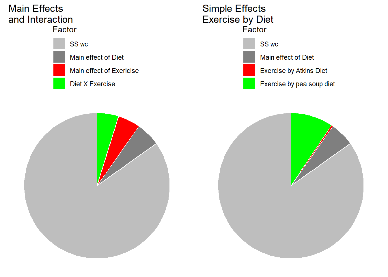
Our simple effects analysis is just another way of breaking down the SS associated with the main effects for columns and the interaction, since the main effect for Diet has no influence on this set of simple effects. You can visualize this by thinking about what would happen to our results of the shapes of the two effects were the same, but if one curve were to be shifted above or below another. For example if our results had come out like this, with an overall higher systolic blood pressure for the Atkins diet:
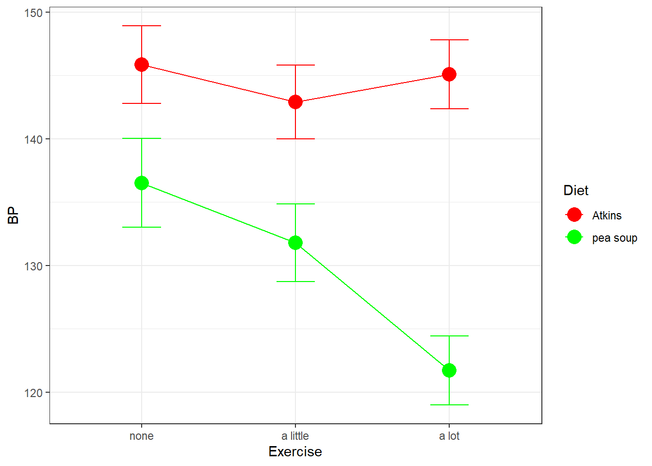
Our simple effects analysis of columns by row would have come out the same. This is because shifting up the Atkins group only increased the main effect of Diet, and not the main effects of Exercise by Diet, the main effect of Exercise, or the interaction between Exercise and Diet.