Chapter 14 \(\chi^{2}\) Test for Independence
This test determines whether the frequencies with which observations fall into two nominal-scale factors are independent of one another.
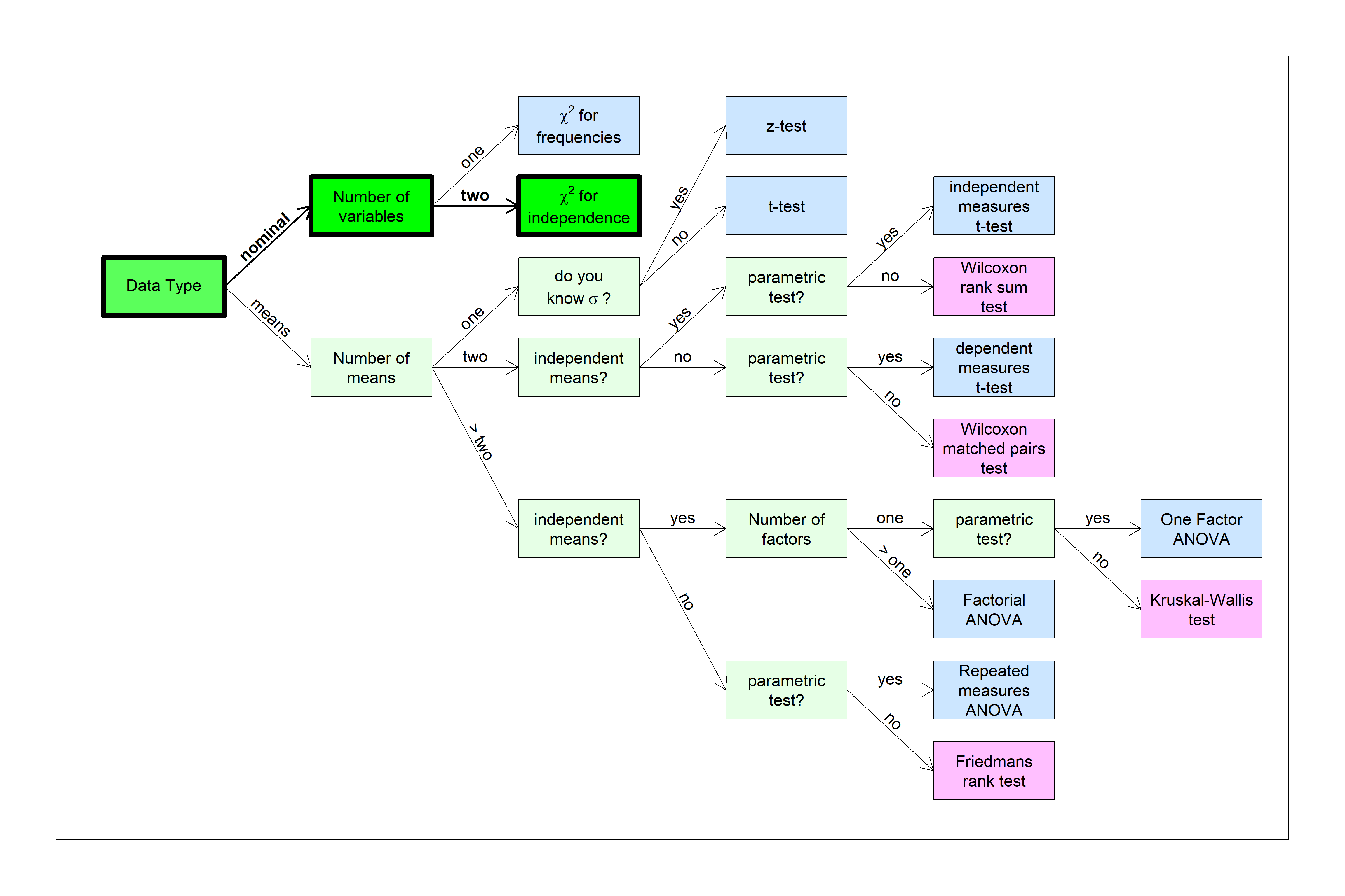
You can find this test in the flow chart here:
For the first example, we’ll use this test to see if the choice of computers that students use varies with gender.
14.1 Example 1: Computer users by gender
To find out we’ll run a \(\chi^{2}\) test for independence using alpha = 0.05.
We’ll use our survey data and count the number of students who use each kind of computer, depending upon their gender. This generates the following 2 X 2 table:
| Apple | PC | |
|---|---|---|
| Women | 82 | 32 |
| Men | 13 | 13 |
If you add up the rows and columns, you’ll see that there are \(82+13 = 95\) students who use Apple computers, and \(32+13 = 45\) students who use PC computers. If computer choice did not depend on gender, then we should see a similar 95/45 ratio of computer use within the subsets of women and men in the class.
This type of frequency data can be visualized with a bar graph with a legend representing the second factor:

By the way, it’s an arbitrary choice for which factor is on the x-axis and which factor is in the legend. Here’s the same data plotted the other way around:
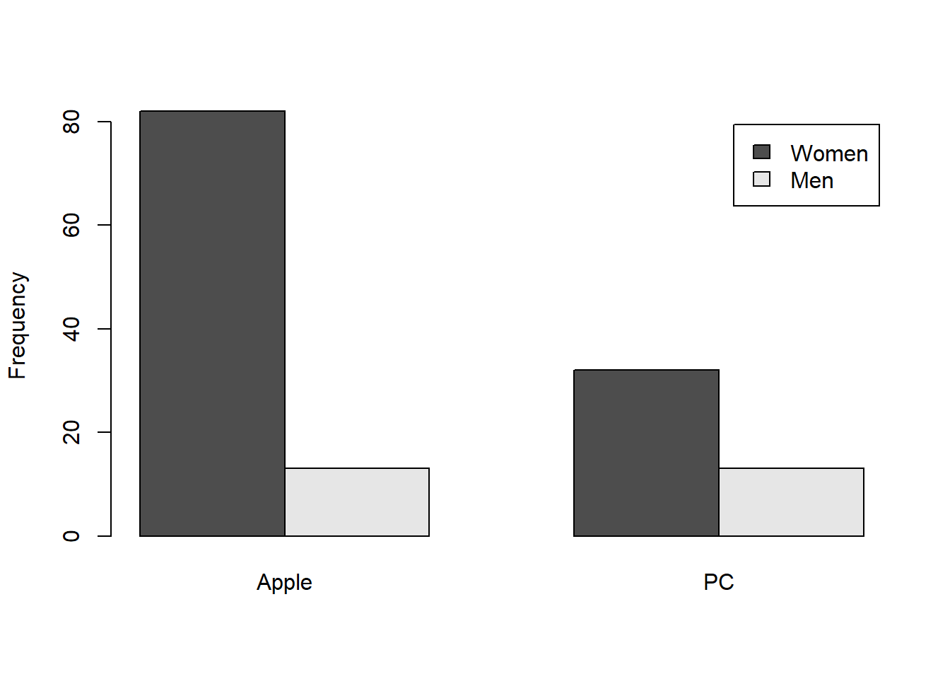
I find it interesting as a vision scientist that you can get different impressions of the data from these two graphs. Typically, for some reason, the implication is that the x-axis factor is causing any difference the legend factor. That’s why the first graph seems more meaningful. It’s more likely that your gender will determine the choice of computer rather than the other way around.
Anyway, to test the null hypothesis that computer use is independent of gender, we generate a table of expected frequencies. This table is set up so that the ratios of computer use are the same within each gender, but also ensures that the ratio of genders is the same across computer use.
An easy way to calculate the table of expected frequencies is to add up the rows and columns for observed frequencies. These are sometimes called marginal sums presumably because we put these numbers in the margins of the table. The total number of observations naturally ends up in the bottom right corner the table:
| Apple | PC | Row Sum | |
|---|---|---|---|
| Women | 82 | 32 | 114 |
| Men | 13 | 13 | 26 |
| Column Sum | 95 | 45 | 140 |
Then, to get the expected frequency for each cell we multiply the sum for that cell’s row with the sum for that cell’s column and divide by the total number of observations:
| Apple | PC | |
|---|---|---|
| Women | \(\frac{(114)(95)}{140} = 77.3571\) | \(\frac{(114)(45)}{140} = 36.6429\) |
| Men | \(\frac{(26)(95)}{140} = 17.6429\) | \(\frac{(26)(45)}{140} = 8.3571\) |
You should convince yourself that these expected frequencies have the right ratios under the null hypothesis. For example, for Women, the expected ratio of Apple to PC computer users is \(\frac{77.3571}{36.6429} = 2.11\). For Men, the ratio is the same:\(\frac{17.6429}{8.3571} = 2.11\). This is the same as the ratio of computer users for the whole class: \(\frac{95}{45} = 2.11\)
Going the other way, for Apple users, the expected ratio of Women to Men is \(\frac{77.3571}{17.6429} = 4.38\). The ratio is the same for PC users: \(\frac{36.6429}{8.3571} = 4.38\). This is the same as the ratio of genders for the whole class: \(\frac{114}{26} = 4.38\)
The math for calculating \(\chi^{2}\) is just like for the \(\chi^{2}\) test for frequencies. For each cell we calculate \(\frac{(f_{obs}-f_{exp})^{2}}{f_{exp}}\) for each cell and sum up across all cells in the matrix:
\[\chi^{2} = \sum{\frac{(f_{obs}-f_{exp})^{2}}{f_{exp}}}\]
Here’s a table for each cell’s \(\chi^{2}\) value:
| Apple | PC | |
|---|---|---|
| Women | \(\frac{(82-77.3571)^{2}}{77.3571} = 0.2787\) | \(\frac{(32-36.6429)^{2}}{36.6429} = 0.5883\) |
| Men | \(\frac{(13-17.6429)^{2}}{17.6429} = 1.2218\) | \(\frac{(13-8.3571)^{2}}{8.3571} = 2.5794\) |
The sum across all cells is \(\chi^{2} = \sum{\frac{(f_{obs}-f_{exp})^{2}}{f_{exp}}} = \frac{(82-77.3571)^{2}}{77.3571} + \frac{(13-17.6429)^{2}}{17.6429} + \frac{(32-36.6429)^{2}}{36.6429} + \frac{(13-8.35714)^{2}}{8.35714} = 4.6681\)
The degrees of freedom for this test is (number of rows - 1)(number of columns - 1) = \(df = (2-1)(2-1) = 1\). You should see that this measure, \(\chi^{2}\), is close to zero when the observed frequencies match the expected frequencies. Therefore, large values of \(\chi^{2}\) can be considered evidence against the null hypothesis of independence.
We can use pchisq to find the p-value for this example:
## [1] 0.0307279We can report our results in APA format like this: “Chi-Squared(1,N=140) = 4.6681, p = 0.0307”.
Using \(\alpha\) = 0.05 we can conclude that the choice of computers is not independent of gender.
14.2 Example 2 Does where you sit in class depend on gender?
When teaching my big classes, I notice that the women tend to sit disproportionately up front and the men in the back. This is a thing? This will be another \(\chi^{2}\) test for independence using alpha = 0.05.
This time we’ll do it using chisq.test straight from the survey data. The first step is to make a table of frequencies.
survey <-read.csv("http://www.courses.washington.edu/psy315/datasets/Psych315W21survey.csv")
dat <- table(survey$gender,survey$sit)
We’re almost there, but there are two issues, first, there are three rows for gender, but the first row - for those who chose not to answer - doesn’t have enough people in it, so we’ll need to leave this row out. The second issue is small - the order of the levels are alphabetical, but it’d be nice to turn them around so they read from front to back. Both of these issues can be fixed by selecting which rows and columns we want in the order that we want.
Tables are really two-dimensional matrices, where the first dimension is the row, and the second dimension is the column. We want to select the second and third row, and re-order the columns so that the second comes first, the first comes second, and the third stays the same. This can be done like this:
##
##         Near the front In the middle Toward the back
##   Man                3            16              10
##   Woman             44            56              22
The easiest way to plot this data is using R’s barplot function. I set beside = TRUE to have the bars for Men and Women next to each other instead of the default which is stacked.

We’re now ready for the \(\chi^{2}\) test, using the same function as the \(\chi^{2}\) test for frequencies:
The output is much like the output for the \(\chi^{2}\) test for frequencies. The expected frequencies are provided as a table, and can be found here:
##
##         Near the front In the middle Toward the back
##   Man          9.02649      13.82781        6.145695
##   Woman       37.97351      58.17219       25.854305
We can extract the information we need to generate a string containing the APA style like we did for the \(\chi^{2}\) test for frequencies:
sprintf('Chi-Squared(%d,N=%d) = %5.4f, p = %5.4f',
        chisq.out$parameter,
        sum(chisq.out$observed),
        chisq.out$statistic,
        chisq.out$p.value)
## [1] "Chi-Squared(2,N=151) = 8.3941, p = 0.0150"So, using \(\alpha\) = 0.05 it looks like where students like to sit in class is not independent of gender.
We have 2 degrees of freedom because we have 2 rows and 3 columns, so \(df = (3-1)(2-1) = 2\).
This test only tells you whether the two factors are independent or not. Typically you need to go back to the table of observations or the plot to make any inferences about what drove a significant result. From this example you can see that the ratio of Men to Women varies from front to back, with a more unbalanced ratio in the front compared to the back. The \(\chi^2\) test for independence tells you how likely it would be to observe deviations from independence at least this large if the two factors were truly independent in the population.
14.3 Effect size and power
Calculating and interpreting effect size is exactly the same as for the \(\chi^{2}\) test for frequencies. \(\psi\) is used for calculating power in R is Cohen’s \(\psi\):
\(\psi = \sqrt{\frac{\chi^{2}}{N}}\)
For our last example \(\psi\) is:
\(\psi = \sqrt{\frac{\chi^{2}}{N}} = \sqrt{\frac{8.3941}{151}} = 0.2358\)
And Cramer’s V is:
\(V =\sqrt{\frac{\chi^{2}}{N \times df}} = \sqrt{\frac{8.3941}{(151)(2)}} = 0.1667\)
Using Cramer’s V, we’d call this a small effect size.
Similarly, power.chisq.test works for the \(\chi^{2}\) test for independence:
Power for the second example is:
## [1] 0.7396396The sample sized needed to get a power of 0.8 is:
## [1] 173.2807